- Home
- About Journals
-
Information for Authors/ReviewersEditorial Policies
Publication Fee
Publication Cycle - Process Flowchart
Online Manuscript Submission and Tracking System
Publishing Ethics and Rectitude
Authorship
Author Benefits
Reviewer Guidelines
Guest Editor Guidelines
Peer Review Workflow
Quick Track Option
Copyediting Services
Bentham Open Membership
Bentham Open Advisory Board
Archiving Policies
Fabricating and Stating False Information
Post Publication Discussions and Corrections
Editorial Management
Advertise With Us
Funding Agencies
Rate List
Kudos
General FAQs
Special Fee Waivers and Discounts
- Contact
- Help
- About Us
- Search


The Open Atmospheric Science Journal
(Discontinued)
ISSN: 1874-2823 ― Volume 14, 2020
Investigation of WRF Microphysics Schemes and Dynamics During an Extreme Precipitation Event in East Idaho
Thomas A. Andretta*
Abstract
Background:
The 26 December 2003 snowstorm was a rare and long-lived weather system that affected east Idaho. Light snow began falling Christmas night, became steadier and heavier during the next day, and tapered off during the morning on the 27th. Snowfall estimates of 20.3-38.1 cm (8.0-15.0 in) were observed over a 24-hour period on 26 December 2003 in the lower part of the Snake River Plain, paralyzing local communities and transportation centers with snowdrifts and poor visibilities.
Methods:
The Weather Research and Forecasting Unified Environmental Modeling System was used to conduct a sensitivity study of five precipitation microphysics schemes at two grid scales during the event.
Results:
A comparison of the model accumulated total grid scale precipitation at 12-km and 4-km scales with the observed precipitation at several stations in the lower plain, indicated small negative biases (underprediction) in all of the schemes. The Purdue-Lin and Weather Research and Forecasting Double-Moment 6-Class microphysics schemes contained the smallest root mean squared errors.
Conclusion:
The Purdue-Lin and Weather Research and Forecasting Double-Moment 6-Class schemes provided several insights into the dynamics of the snowstorm. A topographic convergence zone, seeder-feeder mechanism, and convective instability were major factors contributing to the heavy snowfall in the lower plain.
Article Information

Identifiers and Pagination:
Year: 2018Volume: 12
First Page: 58
Last Page: 79
Publisher Id: TOASCJ-12-58
DOI: 10.2174/1874282301812010058
Article History:
Received Date: 22/3/2018Revision Received Date: 16/5/2018
Acceptance Date: 13/6/2018
Electronic publication date: 29/6/2018
Collection year: 2018
open-access license: This is an open access article distributed under the terms of the Creative Commons Attribution 4.0 International Public License (CC-BY 4.0), a copy of which is available at: https://creativecommons.org/licenses/by/4.0/legalcode. This license permits unrestricted use, distribution, and reproduction in any medium, provided the original author and source are credited.
* Address correspondence to this author at Andretta Innovations LLC, P.O. Box 21057 Cheyenne, WY 82003, USA; Tel: (307)365-4541; E-mail: tndwx89@wmconnect.com
| Open Peer Review Details | |||
|---|---|---|---|
| Manuscript submitted on 22-3-2018 |
Original Manuscript | Investigation of WRF Microphysics Schemes and Dynamics During an Extreme Precipitation Event in East Idaho | |
1. INTRODUCTION
The 26 December 2003 snowstorm brought widespread snowfall to east Idaho. However, the heaviest accumulations of 20.3-38.1 cm (8.0-15.0 in) occurred in the lower part of the Snake River Plain, as reported by several observation stations. This weather system mainly occurred during the day after Christmas, impacting denizens and travelers with periods of light to moderate snow. Blizzard conditions with blowing snow and poor visibilities developed in the evening of the 26th. National Oceanic and Atmospheric Administration (NOAA) National Weather Service (NWS) meteorologists (including this author) issued several winter storm watches and warnings during this life-threatening event. This snowstorm set several snowfall records and is one of the most intriguing winter weather systems to impact east Idaho.
1.1. Motivation of Study
This manuscript explores the dynamics of this snowstorm with observational sources and nested grid high-resolution numerical simulations. This work is motivated to understand the physical processes responsible for locally heavy snowfall in east Idaho as determined by several precipitation microphysics schemes. This research will hopefully benefit the general public, operational weather forecasters, atmospheric modelers, and decision support managers.
The physical processes of the snowstorm will be investigated using high-resolution numerical models, in which one or more variables are perturbed from a given initial state. Accordingly, this manuscript will explore the evolution and structure of the snowstorm in the Weather Research and Forecasting (WRF) Unified Environmental Modeling System (UEMS) [1Skamarock WC, Klemp JB, Dudhia J, et al. A description of the Advanced Research WRF Version 3 2008.] using several precipitation microphysics schemes.
The layout of this paper follows this structure. Section 2 describes the region of study. Section 3 describes the observations in the paper; Section 4 describes the WRF-UEMS grid configuration and design of numerical experiments. Section 5 discusses the results of the numerical simulations of the snowstorm with several precipitation microphysics schemes; Section 6 presents the main conclusions of this manuscript.
1.2. Description of Research Questions
This study addresses several research questions involving the evolution of the snowstorm. What was the performance of several WRF precipitation microphysics schemes at verification points in the lower part of the Snake River Plain? Did the model grid scale and terrain resolution modulate precipitation amounts in these schemes? Based on the most verifiable schemes, what were the physical processes that contributed to the localized heavy snowfall in the lower plain? These research questions are fully addressed in Section 5 of the manuscript.
2. REGION OF STUDY
2.1. Topography
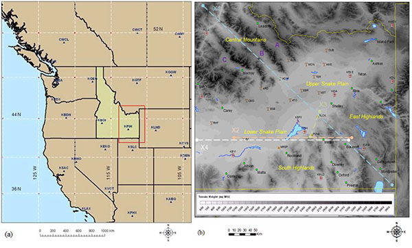
Idaho is a land-locked region in the west United States (Fig. 1a ). The geographical domain of east Idaho is illustrated in Fig. (1b) (red box in Fig. 1a). The Snake River Plain (≈250 km long and ≈100 km wide), curves from the west towards the north-east around the Central Mountains. This plain includes the Lower Snake River Plain and the Upper Snake River Plain. The valley floor gradually ascends from ≈1200 m (all heights above MSL) at the west end of the lower plain to ≈1700 m near the east end of the upper plain. The Snake River Plain is surrounded by several large mountain ranges: the Central Mountains (≈2500–3000 m) to the north-west, the East Highlands (~2500–3000 m) to the east, and South Highlands (≈2000–2500 m) to the south of the plain. The main tributary valleys in the Central Mountains are the Birch Creek (purple label A in Fig. (1b), Little Lost River (B), and Big Lost River (C) valleys.
As Fig. (1b) illustrates, there are four climate stations and verification points (symbols) in the lower plain. Massacre Rocks State Park (MRSP) and Pocatello Regional Airport (KPIH) are situated in an exposed corridor in the lower plain. The city of Pocatello, including the climate station at Pocatello 2 NE (P2NE), is located at the foot of a small mountain range (Portneuf Range) adjoining the South Highlands. The city of Blackfoot (BLCK) is nestled along the foothills of the East Highlands, ≈40 km (25 mi) north-east of Pocatello.
2.2. Precipitation and Snowfall Climatology
Andretta [2Andretta TA. Harmonic analysis of precipitation data in east Idaho. Natl Wea Dig 1999; 23: 31-40.] demonstrated that the Snake River Plain experiences strong second harmonic amplitudes with precipitation maxima in May and November. A third maximum occurs in the winter months between December and March. The tributary valleys and the contiguous Snake Plain are dry topographic features with climatological annual precipitation from 20.30 to 30.50 cm (8.00 to 12.00 in) [3Andretta TA. Forcing, properties, structure, and antecedent synoptic climatology of the Snake River Plain convergence zone of eastern Idaho: Analyses of observations and numerical simulations (Doctor of Philosophy Dissertation) University of Wyoming, Laramie, WY, 2011.]. Furthermore, Andretta and Wojcik [4Andretta TA, Wojcik W. Prediction of heavy snow events in the Snake River Plain using pattern recognition and regression techniques Idaho. NOAA Technical Memorandum NWS WR-268. 2003.] used multiple linear regression techniques to determine that heavy snowfall patterns (≥ 15.2 cm (6.0 in)) occur once per every 1.7 years in the Snake River Plain. This snowstorm also matched the type COLD regression analog pattern in that study, which occurs once per every 2.7 years. Fig. (2a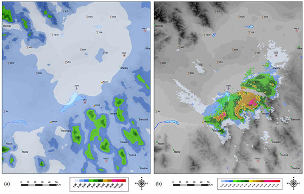 ) shows the Parameter-elevation Relationships on Independent Slopes Model (PRISM) 30-year precipitation normals for the month of December [5Daly C, Halbleib M, Smith JI, et al. Physiographically sensitive mapping of climatological temperature and precipitation across the conterminous United States. Int J Climatol 2008; 28: 2031-64.
[http://dx.doi.org/10.1002/joc.1688] ]. The lower plain typically receives 2.50 to 5.00 cm (1.00 to 2.00 in) of liquid precipitation in the month of December.
2.3. Event Precipitation and Snowfall
Table 1 summarizes the event 24-hour snowfall and snowmelt liquid water equivalent (SWE) collected at reporting times for the four verification points. According to the National Climatic Data Center (NCDC), record snowfall of at least 33.0 cm (13.0 in) (column 3 of table) occurred at KPIH and P2NE. Blackfoot reported the second (tied) highest snowfall of 22.9 cm (9.0 in). The official climate records at KPIH, P2NE, and BLCK were based on 77, 117, and 121 years, respectively. In retrospect, this snow event (≥ 22.9 cm (9.0 in)) was extremely rare, occurring approximately once per every century. Fig. (2b) shows the 24-hour precipitation map for the area based on the KSFX WSR-88D precipitation algorithms. The radar shows local maxima of 0.76 cm (0.30 in) ≈20 km (12 mi) at the east of MRSP and just north-east of P2NE. However, a comparison of Table 1 SWE (column 4 of table) to the liquid amounts in Fig. (2b) suggests that the radar algorithms underestimated the precipitation totals by factors of ≈2.0 at BLCK, ≈4.0 at P2NE, and ≈6.0 at MRSP and KPIH. This discrepancy may arise from topographic beam blockage effects and only horizontal polarization of the falling frozen hydrometeors [3Andretta TA. Forcing, properties, structure, and antecedent synoptic climatology of the Snake River Plain convergence zone of eastern Idaho: Analyses of observations and numerical simulations (Doctor of Philosophy Dissertation) University of Wyoming, Laramie, WY, 2011.]. During this winter event, all the precipitation fell as snow (no rain). Fig. (2a) and Table 1 SWE suggest that these locations received an event SWE equal to at least half of their climatological December values.


3. OBSERVATIONS
3.1. Satellite and In Situ Surface Observations
The NOAA Geostationary Operational Environmental Satellite (GOES) water (H2O) vapor channel (6.5–7.4 µm) is presented in Fig. (3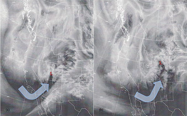 ) at 1130 UTC and 2130 UTC 26 December 2003. This channel measures the amount of water vapor contained in the mid to upper levels (600–100 hPa) of the troposphere [6Weldon RB, Holmes SJ. Water vapor imagery: Interpretation and applications to weather analysis and forecasting. NOAA Technical Report NESDIS 57. 1991.]. In this imagery, white areas indicate deep water vapor content; dark areas denote little or no moisture. The NOAA Forecast Systems Laboratory (FSL) generates the Mesoscale Analysis and Prediction System (MAPS) Surface Assimilation System (MSAS) hourly real-time datasets of analyzed and derived meteorological grids from in situ surface observations [7Miller PA, Barth MF. The AWIPS build 5.2.2 MAPS Surface Assimilation System (MSAS Preprints Interactive Symposium on the Advanced Weather Interactive Processing System (AWIPS) 2002.]. This archived dataset at 1200 UTC and 2100 UTC 26 December 2003 is displayed in Fig. (4
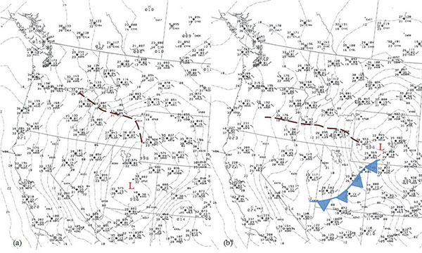 ).
).
Fig. (3a) shows a 600–100 hPa low-pressure system (red “L” symbol) over west Utah with a curved jet stream boundary (light blue arrow) circling the base of the trough over south California and Arizona. The black region was a dry slot of moisture indicating subsidence. A large cloud shield of deep mid to high-level moisture covered most of Nevada, Idaho, and Utah. An intense and closed mean sea-level pressure low (996 hPa) (Fig. 4a: red “L” symbol) was nearly stacked underneath the upper-level cyclone with a zonal surface trough axis (dashed brown line) over central Idaho. By afternoon, the 600–100 hPa cyclone (Fig. 3b) moved into central Wyoming with the moist comma-shaped cloud field covering east Idaho. The jet stream rounded the base of the trough with the dry slot darkening with time, suggesting cyclogenesis (not shown). The MSAS observations (Fig. 4b) showed a 996-hPa low over south-west Wyoming with a surface cold front extending across Utah. Based on the surface observations, snow was falling with sub-freezing temperatures over east Idaho.
 |
Fig. (3) NOAA GOES water vapor imagery at (a) 1130 UTC and (b) 2130 UTC 26 December 2003 with upper-level cyclone (red “L” symbol) and upper-level jet stream (light blue arrow). |

3.2. Doppler Weather Radar Observations
The KSFX Weather Surveillance Radar 88 Doppler (WSR-88D) 0.5° base reflectivity and Mesowest surface observations [8Horel J, Split M, Dunn L, et al. Mesowest: Cooperative mesonets in the western United States. Bull Am Meteorol Soc 2002; 83: 211-25.
[http://dx.doi.org/10.1175/1520-0477(2002)083<0211:MCMITW>2.3.CO;2] ] revealed several interesting meteorological features between 1200 UTC 26 December 2003 and 0600 UTC 27 December 2003 (Fig. 5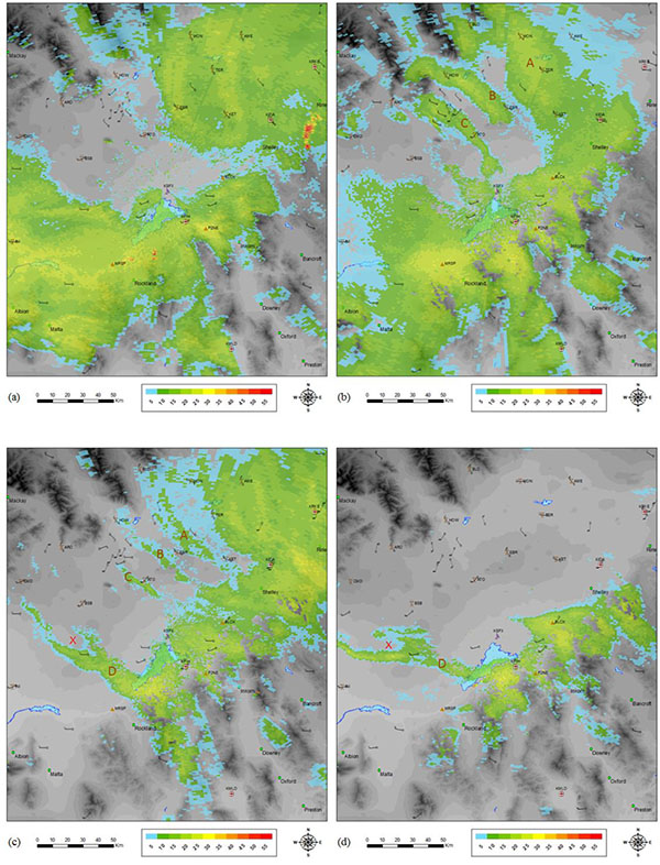 ). During the event, the KSFX WSR-88D was operating in precipitation mode (A) in Volume Coverage Pattern (VCP) 11 (14 elevation scans per every 5 minutes) with a radar reflectivity factor-rainfall rate (Z-R) relationship of Z = 300 R1.4.

At 1200 UTC (Fig. 5a), the radar reflectivity pattern indicated a large area of weak to moderate (10–30 dBZ) echoes associated with the passage of a Pacific cold front in east Idaho. At 1500 UTC (Fig. 5b), a Snake Plain Convergence Zone (SPCZ) formed behind this front as the low-level flow became blocked and converged around the Central Mountains [9Andretta TA, Hazen DS. Doppler radar analysis of a snake river plain convergence event. Weather Forecast 1998; 13: 482-91.
[http://dx.doi.org/10.1175/1520-0434(1998)013<0482:DRAOAS>2.0.CO;2] , 10Andretta TA. Climatology of the snake river plain convergence zone. Natl Wea Dig 2002; 26: 37-51., 3Andretta TA. Forcing, properties, structure, and antecedent synoptic climatology of the Snake River Plain convergence zone of eastern Idaho: Analyses of observations and numerical simulations (Doctor of Philosophy Dissertation) University of Wyoming, Laramie, WY, 2011.]. This SPCZ was identified as three (labels: A, B, C) major reflectivity bands, extending from the exit regions of the tributary valleys to the Upper Snake River Plain. These reflectivity belts generated light to moderate snow from KRXE to KIDA. A large region of weak to moderate echoes (25–35 dBZ) containing light to moderate snow occurred at MRSP and ≈20 km (12 mi) south of KPIH. At the surface, brisk north-west winds of 8-15 m s-1 (15-30 kt) exited the tributary valleys and converged with west to south-west winds of 5-10 m s-1 (10-20 kt) in the lower plain. A “C-shaped” confluence signature [11Wood VT, Brown RA. Single Doppler velocity signature interpretation of nondivergent environmental winds. J Atmos Ocean Technol 1986; 3: 114-28.
[http://dx.doi.org/10.1175/1520-0426(1986)003<0114:SDVSIO>2.0.CO;2] ] was also detected in the low-level radial base velocity data (not shown). At 2100 UTC (Fig. 5c), the three snowbands persisted but became narrower and less intense. A large field of light to moderate snow (15-30 dBZ) was also occurring in the Upper Snake River Plain and East Highlands. A solitary (label: D) snowband extended across the lower plain, producing moderate snow from mesonet site CMD to between MRSP and KPIH. A misocyclone (red “X” symbol) formed at the western edge of this snowband from the cyclonic curvature vorticity in the lee of the Central Mountains [3Andretta TA. Forcing, properties, structure, and antecedent synoptic climatology of the Snake River Plain convergence zone of eastern Idaho: Analyses of observations and numerical simulations (Doctor of Philosophy Dissertation) University of Wyoming, Laramie, WY, 2011., 12Andretta TA. Topographic sensitivity of the snake river plain convergence zone of eastern Idaho: Part II: Numerical simulations. Electronic J Severe Storms Meteor 2014; 9: 1-33.]. At 0600 UTC 27 December 2003 (Fig. 5d), snowband D and the misocyclone persisted with light to moderate echoes (15–35 dBZ) in the lower plain. The strongest echoes occurred near KPIH and BLCK. The convection dissipated after 1200 UTC on the 27th as the atmosphere became drier and more stable.
4. NUMERICAL MODEL
4.1. Description of Numerical Experiments
This section describes the Weather Research and Forecasting (WRF) Unified Environmental Modeling System (UEMS) grid configuration and design of numerical experiments. This WRF-UEMS model (Version 3.7.1) is based on the non-hydrostatic WRF-ARW (Weather Research and Forecasting) model [1Skamarock WC, Klemp JB, Dudhia J, et al. A description of the Advanced Research WRF Version 3 2008.]. Table 2 lists the settings and details of the numerical simulations for the 26 December 2003 event.

As Fig. (6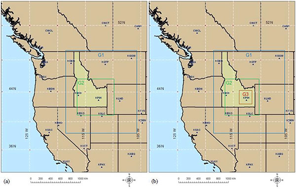 ) illustrates, this study features two WRF-UEMS grid configurations in the simulations. Run A contains grids at 12 and 4 km; Run B contains grids at 12, 4, and 1.33 km. For example, Run B3 refers to Run B at grid 3 (G3: 1.33 km). There is two-way nesting between the outer model grid and inner model nested grids.
The numerical WRF-UEMS simulations used a model spin-up time of ≈12 hours in order to resolve the antecedent, synoptic, and post synoptic-scale environments of the snowstorm. All of the simulations were initialized at 1200 UTC 25 December 2003 and ended at 1200 UTC 27 December 2003, lasting 48 hours. The initial and lateral boundary conditions originated from the 6-hourly North American Regional Reanalysis (NARR) 32-km grids [13Mesinger F, DiMego G, Kalnay E, et al. North American regional reanalysis. Bull Am Meteorol Soc 2006; 87: 343-60.
[http://dx.doi.org/10.1175/BAMS-87-3-343] ]. The model contained 45 vertical levels with a top initialized at 50 hPa and a pressure interval of ΔP = 25 hPa.
 |
Fig. (6) WRF-UEMS model domains (a) Run A: grids G1 (blue) and G2 (green) (12, 4 km), and (b) Run B: grids G1 (blue), G2 (green), and G3 (brown) (12, 4, 1.33 km). |
Model microphysics are divided into bin and bulk categories [14Seifert A, Khain A, Pokrovsky A, Beheng KD. A comparison of spectral bin and two-moment bulk mixed-phase cloud microphysics. Atmos Res 2006; 80: 46-66.
[http://dx.doi.org/10.1016/j.atmosres.2005.06.009] ]. For bin schemes, Particle Size Spectra (PSD) of aerosols and hydrometeors are explicitly resolved requiring abundant computational power. By contrast, for bulk microphysical schemes, PSD is computed directly from measurements [15Henderson D, Mὄlders N. Evaluation of WRF-forecasts over Siberia: Air mass formation, clouds and precipitation. Open Atmos Sci J 2012; 6: 93-110.
[http://dx.doi.org/10.2174/1874282301206010093] , 16Shrestha RK, Connolly PJ, Gallagher MW. Sensitivity of WRF cloud microphysics to simulations of a convective storm over the Nepal Himalayas. Open Atmos Sci J 2017; 11: 29-43.
[http://dx.doi.org/10.2174/1874282301711010029] ]. Single moment bulk schemes predict the mixing ratio of hydrometeors; double moment bulk schemes include another prognostic variable, hydrometeor size distribution, obtained from particle diameter and number concentration. Accordingly, Table 2 shows several bulk microphysics parameterizations in the simulations: Purdue-Lin (PLIN) [17Lin Y-L, Farley RD, Orville HD. Bulk parameterization of the snow field in a cloud model. J Clim Appl Meteorol 1983; 22: 1065-92.
[http://dx.doi.org/10.1175/1520-0450(1983)022<1065:BPOTSF>2.0.CO;2] ], Ferrier or Eta (ETA) [18Ferrier BS, Jin Y, Lin Y, Black T, Rogers E, DiMego G. Implementation of a new grid-scale cloud and precipitation scheme in the NCEP Eta model. 15th conference on numerical weather prediction. Texas: Amer Meteor Soc 2002.], Morrison (MRSN) [19Morrison H, Thompson G, Tatarskii V. Impact of cloud microphysics on the development of trailing stratiform precipitation in a simulated squall line: Comparison of one– and two–moment schemes. Mon Weather Rev 2009; 137: 991-1007.
[http://dx.doi.org/10.1175/2008MWR2556.1] ], Stony Brook University (SBU-YLIN) [20Lin Y, Colle BA. A new bulk microphysical scheme that includes riming intensity and temperature–dependent ice characteristics. Mon Weather Rev 2011; 139: 1013-35.
[http://dx.doi.org/10.1175/2010MWR3293.1] ], and Weather Research and Forecasting (WRF) Double-Moment 6-Class (WDM6) [21Lim K-SS, Hong S-Y. Development of an effective double–moment cloud microphysics scheme with prognostic cloud condensation nuclei (CCN) for weather and climate models. Mon Weather Rev 2010; 138: 1587-612.
[http://dx.doi.org/10.1175/2009MWR2968.1] ]. The PLIN, ETA, SBU-YLIN are single moment bulk schemes; the MRSN and WDM6 are double moment bulk schemes which have exhibited modest skill in simulations of cold clouds over the Himalayas [16Shrestha RK, Connolly PJ, Gallagher MW. Sensitivity of WRF cloud microphysics to simulations of a convective storm over the Nepal Himalayas. Open Atmos Sci J 2017; 11: 29-43.
[http://dx.doi.org/10.2174/1874282301711010029] ]. All of the schemes forecast mixing ratios of water vapor, cloud liquid water, cloud ice, snow, and rain. The SBU-YLIN [20Lin Y, Colle BA. A new bulk microphysical scheme that includes riming intensity and temperature–dependent ice characteristics. Mon Weather Rev 2011; 139: 1013-35.
[http://dx.doi.org/10.1175/2010MWR3293.1] ] and WDM6 [21Lim K-SS, Hong S-Y. Development of an effective double–moment cloud microphysics scheme with prognostic cloud condensation nuclei (CCN) for weather and climate models. Mon Weather Rev 2010; 138: 1587-612.
[http://dx.doi.org/10.1175/2009MWR2968.1] ] schemes provide advanced hydrometeor predictions. In particular, the WDM6 scheme includes cloud condensation nuclei concentration, particle size spectra of cloud liquid water and rain, and graupel mixing ratio. The SBU-YLIN scheme substitutes graupel with precipitating ice, a function of riming intensity and temperature. These schemes will provide new insights into frozen precipitation during the 26 December 2003 winter storm over the complex terrain of east Idaho. A study from this perspective hasn’t yet been reported in the literature and will be extremely valuable to the general public, operational weather forecasters, atmospheric modelers, and decision support managers.
Boundary layer parameterizations in this study include the Mellor-Yamada-Janjić (MYJ) [22Mellor GL, Yamada T. Development of a turbulence closure model for geophysical fluid problems. Rev Geophys Space Phys 1982; 20: 851-75.
[http://dx.doi.org/10.1029/RG020i004p00851] , 23Janjić ZI. Nonsingular implementation of the Mellor-Yamada level 2.5 scheme in the NCEP Meso model. NCEP Office Note No. 437. 2002.] scheme. Numerical modelers use the cumulus convective scheme at coarse grid scales ≥ 4 km [24Kain JS. The Kain–Fritsch convective parameterization: An update. J Appl Meteorol 2004; 43: 170-81.
[http://dx.doi.org/10.1175/1520-0450(2004)043<0170:TKCPAU>2.0.CO;2] , 25Kain JS, Weiss SJ, Levit JJ, Baldwin ME, Bright DR. Examination of convection-allowing configurations of the WRF model for the prediction of severe convective weather: The SPC/NSSL Spring Program 2004. Weather Forecast 2006; 21: 167-81.
[http://dx.doi.org/10.1175/WAF906.1] ]. Hence, the convective scheme was activated in grids A1, A2, B1, and B2. The cumulus parameterization was deactivated in Run B with grid 3 so the model could explicitly resolve cumulus clouds at finer grid scales of 1.33 km [1Skamarock WC, Klemp JB, Dudhia J, et al. A description of the Advanced Research WRF Version 3 2008.].
4.2. Types of Sensitivity Experiments
There are two categories of sensitivity experiments. In each test, all other variables remained constant during the simulation. For reference, Table 2 shows the specific model settings subject to the sensitivity tests. In the first category, Runs A and B were conducted at two different grid scales (Fig. 6) and topographic resolutions. Second, the physical processes of the snowstorm were investigated in which a single simulation was conducted with a specific precipitation microphysics scheme. There were a total of eight sensitivity experiments within this category using the different microphysics schemes. In particular, Run A included five simulations with all of the schemes (Table 2). Run B contained three simulations with these schemes: PLIN, SBU-YLIN, and WDM6. These decisions and their outcomes will be discussed further in the next section of the manuscript.
5. RESULTS AND DISCUSSION
5.1. Comparison of Model to Observations
The synoptic pattern is illustrated in Fig. (7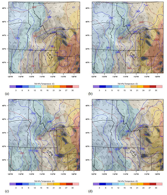 ) at four time steps in the WRF-UEMS model (Run A1). At 1200 UTC (Fig. 7a), the meridionally elongated closed cyclones at 700 hPa and mean sea-level were almost vertically stacked over north-east Utah and west Wyoming. The model generally agreed with the surface observations Fig. (4a) in location and intensity (995 hPa) of the mean sea-level pressure low. The horizontal zonal temperature gradient at 700 hPa was ≈−10 °C (cooling) with a horizontal zonal pressure gradient [26Holton JR. An Introduction to Dynamic Meteorology 2004.] of ≈14 hPa across south Idaho. At 1500 UTC (Fig. 7b), the 700-hPa and surface cyclones remained nearly stationary with a trough axis forming across Central Mountains and Upper Snake River Plain. The horizontal pressure gradient across south Idaho strengthened to ≈18 hPa. At 1800 UTC (Fig. 7c), the 10-m AGL winds intensified under this tight pressure gradient with north-west winds of 10–15 m s-1 (20–30 kt) exiting the tributary valleys and converging with west to south-west winds of 5–12 m s-1 (10–25 kt) in the lower plain. The model correctly reproduced this surface convergence wind field in the observations (Fig. 5b). At 2100 UTC (Fig. 7d), the model mean sea-level pressure low (997 hPa) was slightly west of the observations (Fig. 4b); the horizontal pressure gradient weakened slightly (≈15 hPa) across south Idaho in both the model and observations.
5.2. Precipitation Microphysics Schemes
This section explores the performance of five precipitation microphysics schemes (PLIN, ETA, MRSN, SBU-YLIN, and WDM6) in the WRF-UEMS model at the four verification sites (MRSP, KPIH, P2NE, and BLCK) in the lower plain (Table 1, Fig. 1b). The closest model grid points were selected for the locations of the verification points. Table 3 (Run A2) and Table 4 (Run B3) summarize the bias (BIAS) and Root Mean Squared Error (RMSE) statistics [27Wilks DS. Statistical Methods in the Atmospheric Sciences 2006.] for the precipitation in the five microphysics schemes.


The equations for the BIAS (1) and RMSE (2) are given for the N = 4 observations, as:
 |
(1) |
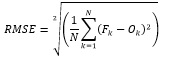 |
(2) |
where,
k: kth observation station (MRSP, KPIH, P2NE, BLCK)
Fk: WRF-UEMS grid-scale precipitation at grid point (i, j) closest to station k (latitude, longitude)
Ok: NCDC observation of precipitation at station k

The first objective is to investigate the role of finer grid spacing and terrain resolution on the precipitation output in the five schemes, comparing the accumulated total grid-scale precipitation in Run A2 (4 km) (Fig. 8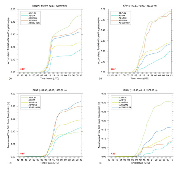 ) with Run B3 (1.33 km) (Fig. 9
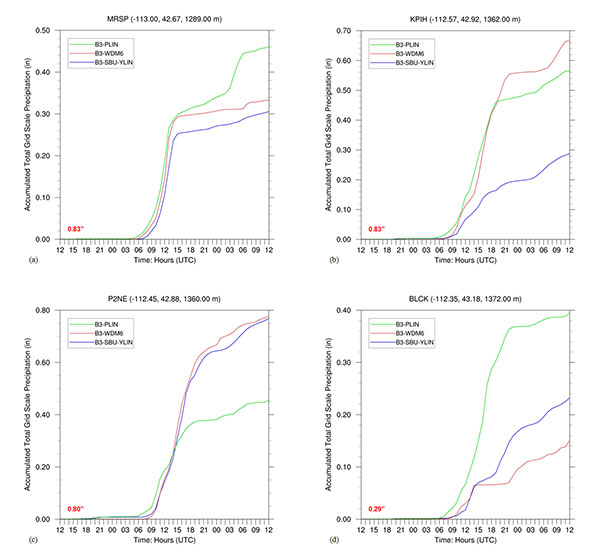 ) at the four verification points. For reference, the 24-hour observed SWE (Table 1: column 3) is indicated in bold red text in the lower left of the figures. In Run A2, all of the schemes under-predicted the precipitation (Table 3) with slight negative biases (Fig. 8a). The PLIN scheme performed best at BLCK (Fig. 8d); the PLIN and WDM6 schemes were nearly equal (≈1.45 cm or 0.57 in) and closer to observations at KPIH (Fig. 8b), 2.11 cm (0.83 in); the SBU-YLIN and WDM6 schemes were nearly tied (≈2.16 cm or 0.85 in) at P2NE (Fig. 8c). The ETA and MRSN schemes in Figs. (8a-d) grossly underpredicted the accumulated total grid-scale precipitation at all four sites in the A2 simulation with root mean squared errors between 0.40 and 0.50.
 |
Fig. (8) WRF-UEMS Run A2 accumulated total grid scale precipitation (in) using PLIN (solid green line), ETA (solid aqua line), MRSN (solid yellow line), WDM6 (solid brown line), and SBU-YLIN (solid blue line) schemes at (a) MRSP, (b) KPIH, (c) P2NE, and (d) BLCK. The 24-hour observed SWE (bold red text: in) from Table 1 is indicated in the lower left of the figures. The longitude (decimal degrees), latitude (decimal degrees), and station elevation (m MSL) are indicated at the top of the figures. The model run cycle is 48-hours from 1200 UTC 25 December 2003 to 1200 UTC 27 December 2003. |
 |
Fig. (9) WRF-UEMS Run B3 accumulated total grid-scale precipitation (in) using PLIN (solid green line), WDM6 (solid red line), and SBU-YLIN (solid blue line) schemes at (a) MRSP, (b) KPIH, (c) P2NE, and (d) BLCK. The 24-hour observed SWE (bold red text: in) from Table 1 is indicated in the lower left of the figures. The longitude (decimal degrees), latitude (decimal degrees), and station elevation (m MSL) are indicated at the top of the figures. The model run cycle is 48-hours from 1200 UTC 25 December 2003 to 1200 UTC 27 December 2003. |
In Run B3, both schemes under-forecasted the precipitation (Table 4) with small negative biases and root mean squared errors (≈0.30). At the finer grid scale and topographic resolution in Run B3, the PLIN scheme was closer to the observations at MRSP (Fig. 9a) and BLCK (Fig. 9d); the WDM6 scheme performed better at KPIH (Fig. 9b) and nearly the same at P2NE (Fig. 9c) versus Run A2. The SBU-YLIN scheme verified extremely well at P2NE (Figs. 8c, 9c) in both simulations but consistently underperformed elsewhere. In sum, the sensitivity tests with Runs A2 and B3 suggest that the PLIN and WDM6 schemes performed better at the four stations.
The next analysis in Fig. (10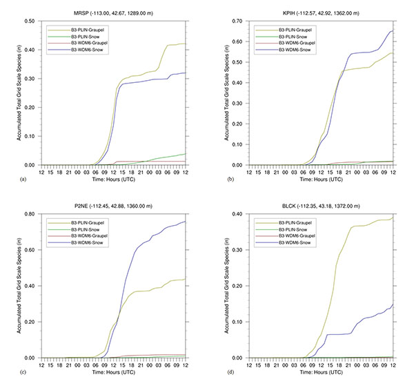 ) explores the partitioning of the accumulated total grid-scale precipitation between graupel and snow plus ice in the PLIN and WDM6 schemes. At MRSP (Fig. 10a), the PLIN and WDM6 schemes indicated similar amounts of graupel and snow, respectively, between 0600 and 2300 UTC 26 December 2003. There were greater differences in the species during the evening hours of the 26th. At BLCK (Fig. 10d), the PLIN scheme generated most of the surface precipitation as graupel instead of snow because of the higher terminal velocities of graupel in the scheme. By contrast, at KPIH (Fig. 10b) and P2NE (Fig. 10c), the WDM6 scheme generated the majority of the surface precipitation as snow. The PLIN scheme produced mostly graupel at P2NE but was outperformed by the WDM6 scheme (Fig. 9c) there. Between 0600 and 1800 UTC, model graupel increased sharply to local maxima of 0.94 cm (0.37 in) at P2NE and BLCK, with only small increases in the afternoon and evening hours of the 26th. The next section examines the physical processes that generated the snow at MRSP, KPIH, and P2NE and the graupel at BLCK.

5.3. Physical Processes
In order to understand the physical processes associated with the precipitation microphysics schemes in this snowstorm, the larger-scale dynamics are explored followed by smaller-scale processes. The WDM6 scheme was arbitrarily selected for this initial analysis. Accordingly, Fig. (11a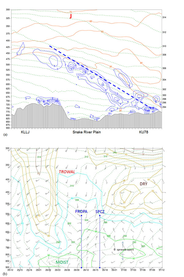 ) shows the synoptic-scale frontogenesis function in a cross-section (Fig. 11b): X1) bisecting the Snake River Plain. As Fig. (1b) illustrates, this transect passes near the surface observations at KLLJ and KU78. The frontal surface and isentropes tilted south-east with the colder air across the Central Mountains. The axis of the cold front (thick dashed blue line) and location of the 325-hPa wind speed maximum (red “J” symbol) are indicated in the transect. A meteogram (Fig. 11b) at KPIH reveals other details. The trough of warm air aloft (trowal) was overhead between 0300 and 0600 UTC 26 December 2003. Meanwhile, the cold front passed KPIH at ≈1000 UTC with a mesoscale SPCZ [3Andretta TA. Forcing, properties, structure, and antecedent synoptic climatology of the Snake River Plain convergence zone of eastern Idaho: Analyses of observations and numerical simulations (Doctor of Philosophy Dissertation) University of Wyoming, Laramie, WY, 2011.] forming behind it at ≈1600 UTC on the 26th. A deep layer of moist air (850-650 hPa) was present during most of the day. The isentropes moved apart between 1600 and 2300 UTC 26 December 2003, indicating the persistence of the SPCZ. Dry air aloft (550-300 hPa) intruded over the airport in the evening hours of the 26th.
 |
Fig. (11) (a) WRF-UEMS Run B2 (WDM6 scheme) at 0900 UTC 26 December 2003 cross-section X1 in Fig. 1b . Frontogenesis function (solid blue contours with blue labels: K [100 km]-1 [3 hr]-1), potential temperature (dashed green contours with black labels: K), and wind speed (solid brown contours with brown labels: kt). The horizontal (transect distance: 450 km) and vertical (pressure: hPa) axes are displayed in the figure. (b) WRF-UEMS Run B3 (WDM6 scheme) meteogram at KPIH with relative humidity (solid color contours with color labels: %), potential temperature (dashed green contours with green labels: K), and wind barbs (black: kt). Each full wind barb is 5 m s-1 (10 kt) and flag is 25 m s-1 (50 kt). The annotations are described in the text. The horizontal (time: UTC date/hour) and vertical (pressure: hPa) axes are displayed in the figure. The model run cycle is 48-hours from 1200 UTC 25 December 2003 to 1200 UTC 27 December 2003.
|
The evolution of the frozen hydrometeors (total of snow and graupel mixing ratios) is shown in Fig. (12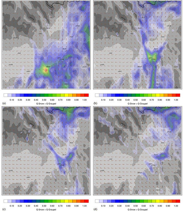 ) using the WDM6 scheme at four model time steps on 26 December 2003. As noted in Fig. (10), the frozen hydrometeors in this scheme were mainly in the form of snow at the four sites. At 1200 UTC (Fig. 12a), there was a well-defined band of snow and graupel associated with the cold front extending from KRXE to KBYI. A local snow mixing ratio maximum (0.06-0.10 g kg-1) was located just south of MRSP. At 1500 UTC (Fig. 12b), a post-cold-frontal topographic convergence zone formed [3Andretta TA. Forcing, properties, structure, and antecedent synoptic climatology of the Snake River Plain convergence zone of eastern Idaho: Analyses of observations and numerical simulations (Doctor of Philosophy Dissertation) University of Wyoming, Laramie, WY, 2011.] in the Snake River Plain. At the surface, brisk north-west winds of 8-15 m s-1 (15-30 kt) exiting the tributary valleys converged with west to south-west winds of 5-10 m s-1 (10-20 kt) in the lower plain. This SPCZ produced several snow mixing ratio maxima (0.04-0.08 g kg-1) at KPIH and P2NE. At 1800 UTC (Fig. 12c), there were several narrow bands of snow and graupel aligned from the exit regions of the tributary valleys to the upper and lower plains. Within this converging air mass, the largest snow mixing ratio maxima (0.02-0.06 g kg-1) occurred at KPIH, P2NE, and just at the east of BLCK. At 2100 UTC (Fig. 12d), these hydrometeor bands weakened in intensity and coverage. However, upslope and converging flows generated a snow mixing ratio maximum (0.02-0.06 g kg-1) near BLCK.

In addition, Figs. (13a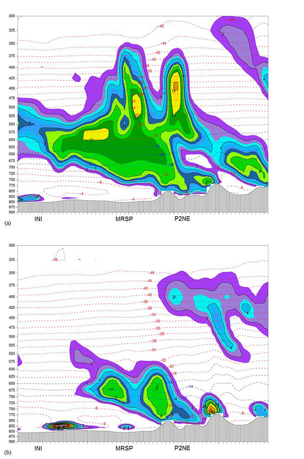 , 13b) show the evolution of a seeder-feeder mechanism [28Rogers RR, Yau MK. A Short Course in Cloud Physics 1989.] in the WDM6 scheme along a cross-section (Fig. 1b): X2). This transect follows a west to an east line from mesonet site INI to near MRSP to 60 km (37 mi) east of P2NE. The times are 1500 and 2100 UTC 26 December 2003. At 1500 UTC (Fig. 13a), a seeder layer of cloud ice water was present from 600 to 350 hPa. This ice fell into a warmer layer of supercooled liquid water below (700-600 hPa) resulting in a mixed-phase cloud. Since the water vapor pressure difference over supercooled liquid water and ice reaches a maximum from −12°C to −16°C, the cloud ice water grew rapidly at the expense of the supercooled liquid water in this thermal layer [28Rogers RR, Yau MK. A Short Course in Cloud Physics 1989.]. During this Wegener-Bergeron-Findeisen process, the feeder layer was the focus of heavy snowfall that occurred near MRSP and P2NE in the morning and afternoon hours (Fig. 13b). Accordingly, as Figs. (13c, d) indicate, high snow mixing ratios (0.02-0.05 g kg-1) with broad vertical ascent (−10 ≥ ω ≥ −20 Pa s-1) occurred within the −12 to −16 °C dendritic layer from north-east of MRSP to the west of P2NE. The rising vertical motions (−2 ≥ ω ≥ −6 Pa s-1) near P2NE suggest upslope flow with snow mixing ratio maxima (0.02-0.05 g kg -1). This seeder-feeder mechanism gradually weakened over the next 6 hours, ending at 2100 UTC.
 |
Fig. (13) WRF-UEMS Run B3 (WDM6 scheme) cross-section X2 in Fig. (1b ) at (a) 1500 UTC and (b) 2100 UTC 26 December 2003 with sum of liquid and ice water mixing ratios (filled colors with solid black contours and black labels: 10-3 g kg-1) and temperature (dashed red contours and labels: ºC); (c) 1500 UTC and (d) 2100 UTC 26 December 2003 with snow mixing ratio (filled colors with solid black contours and black labels: 10-3 g kg-1), temperature (dashed red contours and labels: ºC), and positive vertical velocity (ω < 0: solid purple contours and labels: Pa s-1). The dendritic (−12 to −16 °C) layer is the region of dashed blue isotherms and labels. The horizontal (transect: 220 km) and vertical (pressure: hPa) axes are displayed in the figures.
|
There were also several smaller-scale dynamical processes occurring in this event. Fig. (14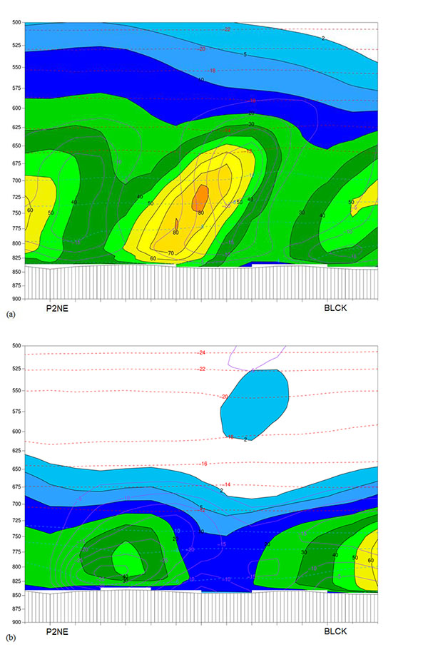 ) shows significant riming in the PLIN scheme in a cross-section (Fig. 1b): X3) from P2NE to BLCK. In this mixed-phase cloud process, falling supercooled liquid water droplets contacted and froze on the surface of the ice crystals in the 0 to −10 °C thermal layer [28Rogers RR, Yau MK. A Short Course in Cloud Physics 1989.]. This ice accretion mainly occurred between 1200 and 1800 UTC 26 December 2003 (Figs. 10c, d). The graupel mixing ratios (0.04–0.08 g kg-1) were largest from just north-east of P2NE to BLCK in this thermal layer with broad vertical ascent (−5 ≥ ω ≥ −35 Pa s-1). In brief, this riming process may explain the heavy snowfall reported at BLCK (Table 1: column 3).
 |
Fig. (14) WRF-UEMS Run B3 (Purde-Lin scheme) cross-section X3 in Fig. 1b at (a) 1200 UTC and (b) 1800 UTC 26 December 2003 with graupel mixing ratio (filled colors with solid black contours and black labels: 10-3 g kg-1), temperature (dashed red contours and labels: ºC), and positive vertical velocity (ω < 0: solid purple contours and labels: Pa s-1). The riming (0 to −10 °C) layer is the region of dashed blue isotherms and labels. The horizontal (transect: 50 km) and vertical (pressure: hPa) axes are displayed in the figures.
|
Fig. (15 ) shows the evolution of nocturnal convection in a cross-section (Fig. 1b): X4). This transect follows a west to east line from 80 km (50 mi) west of mesonet site INI to near MRSP to 60 km (37 mi) east of P2NE. The three model time steps are 0000, 0600, and 1200 UTC 27 December 2003. Convective cells (A and B) contained narrow updrafts (−3 ≥ ω ≥ −9 Pa s-1) along the transect. These upright cells produced snow mixing ratio maxima (0.02-0.08 g kg-1) in an environment of convective instability [28Rogers RR, Yau MK. A Short Course in Cloud Physics 1989.] with the moist isentropes bending and folding over near the ground from INI to just north of MRSP. The figures illustrate a prevailing trend at all three model time steps along the transect: ascending (up grey arrows) cold air and descending (down grey arrows) warm air west of cell A, ascending cold air in between the cells, and descending warm air east of cell B. Hence, these patterns suggest thermally-indirect circulations along the transect. These local circulations may have released the convective instability, allowing these cells to grow and persist during the nocturnal hours. The cells generated heavy snow squalls and blizzard conditions from MRSP to P2NE, as suggested in the surface wind and radar reflectivity observations (Fig. 5d). After 1200 UTC, the airmass became drier and more stable across the Snake River Plain ending the last dynamics of this unique snowstorm.
 |
Fig. (15) WRF-UEMS Run B2 (WDM6 scheme) cross-section X4 in Fig. (1b ) (a) 0000 UTC, (b) 0600 UTC, and (c) 1200 UTC 27 December 2003 with snow mixing ratio (filled colors with solid black contours and black labels: 10-3 g kg-1), equivalent potential temperature (dashed green contours: oK), and vertical velocity (ω < 0: solid purple contours and labels: Pa s-1; ω > 0: dashed pink contours and labels: Pa s-1). The grey arrows with blue outlines show the direction of the vertical motion fields. The horizontal (transect: 270 km) and vertical (pressure: hPa) axes are displayed in the figures.
|
CONCLUSION
The 26 December 2003 snowstorm was a rare and long-lived weather system that affected east Idaho. The heaviest accumulations of 20.3-38.1 cm (8.0-15.0 in) occurred in a relatively small region of the Lower Snake River Plain. This snowstorm surpassed daily snowfall accumulations based on approximately 100-year records at the Pocatello airport and city of Pocatello.
A sensitivity experiment of five WRF-UEMS microphysics schemes resulted in the PLIN and WDM6 schemes performing better at four verification points in the lower plain. These particular schemes provided many insights into the physical processes which generated the locally heavy snowfall. First, the morning synoptic environment featured passage of a Pacific cold front with nearly vertically stacked low-pressure systems moving from west Utah to west Wyoming. The WDM6 scheme showed the transition from this synoptic-scale pattern to a mesoscale terrain-induced convergence zone and seeder-feeder mechanism, both of which produced significant snowfall at MRSP, KPIH, and P2NE. By comparison, the PLIN scheme indicated significant riming (graupel) with broad vertical ascent between P2NE and BLCK. Finally, as indicated in the WDM6 scheme, narrow upright convective cells with thermally-indirect circulations formed in a nocturnal environment of convective instability. These cells generated heavy snow squalls in the lower plain.
CONSENT FOR PUBLICATION
Not applicable.
CONFLICT OF INTEREST
The author declares no conflict of interest, financial or otherwise.
ACKNOWLEDGEMENTS
The author appreciates comments from Dr. Sultan Hameed at Stony Brook University and other reviewers. The author would also like to thank NWS staff meteorologists for their collaboration during this snowstorm, and dedication to saving lives and protecting property.
REFERENCES
| [1] | Skamarock WC, Klemp JB, Dudhia J, et al. A description of the Advanced Research WRF Version 3 2008. |
| [2] | Andretta TA. Harmonic analysis of precipitation data in east Idaho. Natl Wea Dig 1999; 23: 31-40. |
| [3] | Andretta TA. Forcing, properties, structure, and antecedent synoptic climatology of the Snake River Plain convergence zone of eastern Idaho: Analyses of observations and numerical simulations (Doctor of Philosophy Dissertation) University of Wyoming, Laramie, WY, 2011. |
| [4] | Andretta TA, Wojcik W. Prediction of heavy snow events in the Snake River Plain using pattern recognition and regression techniques Idaho. NOAA Technical Memorandum NWS WR-268. 2003. |
| [5] | Daly C, Halbleib M, Smith JI, et al. Physiographically sensitive mapping of climatological temperature and precipitation across the conterminous United States. Int J Climatol 2008; 28: 2031-64. [http://dx.doi.org/10.1002/joc.1688] |
| [6] | Weldon RB, Holmes SJ. Water vapor imagery: Interpretation and applications to weather analysis and forecasting. NOAA Technical Report NESDIS 57. 1991. |
| [7] | Miller PA, Barth MF. The AWIPS build 5.2.2 MAPS Surface Assimilation System (MSAS Preprints Interactive Symposium on the Advanced Weather Interactive Processing System (AWIPS) 2002. |
| [8] | Horel J, Split M, Dunn L, et al. Mesowest: Cooperative mesonets in the western United States. Bull Am Meteorol Soc 2002; 83: 211-25. [http://dx.doi.org/10.1175/1520-0477(2002)083<0211:MCMITW>2.3.CO;2] |
| [9] | Andretta TA, Hazen DS. Doppler radar analysis of a snake river plain convergence event. Weather Forecast 1998; 13: 482-91. [http://dx.doi.org/10.1175/1520-0434(1998)013<0482:DRAOAS>2.0.CO;2] |
| [10] | Andretta TA. Climatology of the snake river plain convergence zone. Natl Wea Dig 2002; 26: 37-51. |
| [11] | Wood VT, Brown RA. Single Doppler velocity signature interpretation of nondivergent environmental winds. J Atmos Ocean Technol 1986; 3: 114-28. [http://dx.doi.org/10.1175/1520-0426(1986)003<0114:SDVSIO>2.0.CO;2] |
| [12] | Andretta TA. Topographic sensitivity of the snake river plain convergence zone of eastern Idaho: Part II: Numerical simulations. Electronic J Severe Storms Meteor 2014; 9: 1-33. |
| [13] | Mesinger F, DiMego G, Kalnay E, et al. North American regional reanalysis. Bull Am Meteorol Soc 2006; 87: 343-60. [http://dx.doi.org/10.1175/BAMS-87-3-343] |
| [14] | Seifert A, Khain A, Pokrovsky A, Beheng KD. A comparison of spectral bin and two-moment bulk mixed-phase cloud microphysics. Atmos Res 2006; 80: 46-66. [http://dx.doi.org/10.1016/j.atmosres.2005.06.009] |
| [15] | Henderson D, Mὄlders N. Evaluation of WRF-forecasts over Siberia: Air mass formation, clouds and precipitation. Open Atmos Sci J 2012; 6: 93-110. [http://dx.doi.org/10.2174/1874282301206010093] |
| [16] | Shrestha RK, Connolly PJ, Gallagher MW. Sensitivity of WRF cloud microphysics to simulations of a convective storm over the Nepal Himalayas. Open Atmos Sci J 2017; 11: 29-43. [http://dx.doi.org/10.2174/1874282301711010029] |
| [17] | Lin Y-L, Farley RD, Orville HD. Bulk parameterization of the snow field in a cloud model. J Clim Appl Meteorol 1983; 22: 1065-92. [http://dx.doi.org/10.1175/1520-0450(1983)022<1065:BPOTSF>2.0.CO;2] |
| [18] | Ferrier BS, Jin Y, Lin Y, Black T, Rogers E, DiMego G. Implementation of a new grid-scale cloud and precipitation scheme in the NCEP Eta model. 15th conference on numerical weather prediction. Texas: Amer Meteor Soc 2002. |
| [19] | Morrison H, Thompson G, Tatarskii V. Impact of cloud microphysics on the development of trailing stratiform precipitation in a simulated squall line: Comparison of one– and two–moment schemes. Mon Weather Rev 2009; 137: 991-1007. [http://dx.doi.org/10.1175/2008MWR2556.1] |
| [20] | Lin Y, Colle BA. A new bulk microphysical scheme that includes riming intensity and temperature–dependent ice characteristics. Mon Weather Rev 2011; 139: 1013-35. [http://dx.doi.org/10.1175/2010MWR3293.1] |
| [21] | Lim K-SS, Hong S-Y. Development of an effective double–moment cloud microphysics scheme with prognostic cloud condensation nuclei (CCN) for weather and climate models. Mon Weather Rev 2010; 138: 1587-612. [http://dx.doi.org/10.1175/2009MWR2968.1] |
| [22] | Mellor GL, Yamada T. Development of a turbulence closure model for geophysical fluid problems. Rev Geophys Space Phys 1982; 20: 851-75. [http://dx.doi.org/10.1029/RG020i004p00851] |
| [23] | Janjić ZI. Nonsingular implementation of the Mellor-Yamada level 2.5 scheme in the NCEP Meso model. NCEP Office Note No. 437. 2002. |
| [24] | Kain JS. The Kain–Fritsch convective parameterization: An update. J Appl Meteorol 2004; 43: 170-81. [http://dx.doi.org/10.1175/1520-0450(2004)043<0170:TKCPAU>2.0.CO;2] |
| [25] | Kain JS, Weiss SJ, Levit JJ, Baldwin ME, Bright DR. Examination of convection-allowing configurations of the WRF model for the prediction of severe convective weather: The SPC/NSSL Spring Program 2004. Weather Forecast 2006; 21: 167-81. [http://dx.doi.org/10.1175/WAF906.1] |
| [26] | Holton JR. An Introduction to Dynamic Meteorology 2004. |
| [27] | Wilks DS. Statistical Methods in the Atmospheric Sciences 2006. |
| [28] | Rogers RR, Yau MK. A Short Course in Cloud Physics 1989. |