Commercially pure titanium discs (Grade IV) with turned surface were used as initial material. The samples (diameter 6.25 mm) were marked with a milled cross creating four quadrants with one of the quadrants marked for visual separation. This made it possible to perform topographical measurements on the same spot after sequential processing steps. In total, three different samples were used in this study where five different surfaces were analysed (Fig. 1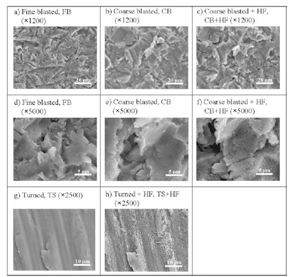). i) turned surface (TS), ii) TS surface treated with diluted hydrofluoric acid (TS+HF), iii) TS blasted with small TiO₂ particles, i.e. fine blasted surface (FB), representing the surface of the previously commercially available TiOblast™ implant (AstraTech AB), iv) TS surface blasted with large TiO₂ particles, i.e. coarse blasted surface (CB), v) CB surface treated with diluted HF (CB+HF), representing the surface of the commercially available dental implant OsseoSpeed™ (AstraTech AB).

Fig. (1) SEM images of the different surfaces. (a-c) show the blasted surfaces at ×1200 magnification while (d-f) show the same surfaces at ×5000 magnification. g) and h) show the turned and etched surfaces at ×2500 magnification.

The TS and CB surfaces were used as references for the TS+HF and CB+HF surfaces, respectively. The HF treatment was performed according to the OsseoSpeed™ process which introduces a smaller topographic structure on top of the underlying surface (Fig. 1). The samples were created and analysed according to the scheme shown in Fig. (2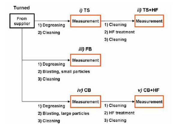), where the TS surface was first analysed and then transformed into the TS+HF surface by the HF treatment. In the same way the CB surface was first analysed and transformed into the CB+HF surface. The influence of the cleaning processes on the topography was investigated and no changes in the surface parameters could be seen. Three points per surface were analysed after each treatment. To follow the topographical changes, area analysis was performed on approximately the same spot after each treatment. On the turned samples (TS, TS+HF), finding the same point was straight forward but more difficult on the blasted surfaces. However, approximately the same points were analysed also on the blasted samples. By performing topographical measurements at the same point after each processing step, detailed information on how each step influences the topography was obtained.

Fig. (2) Scheme over the preparation and measurement process.

To measure both topography from underlying structure together with the topography introduced by the HF-treatment, two different surface sensitive techniques were used; Atomic Force Microscopy (AFM) and 3D-Scanning Electron Microscopy (3D-SEM). The data obtained were imported into the calculation software MeX^® [38], where 3D-roughness parameters were calculated (further discussed in section 3). The MeX^® software is designed to calculate surface roughness parameters from SEM images but was utilised in this work also for analysing AFM data to avoid any differences depending on the software used.

AFM measurements were performed on a Nanoscope^® IIIa (Digital Instruments) equipped with Nanoscope^® 5.12 software, using Tapping Mode. AFM measurements were only possible on the TS and TS+HF samples because of limitations in maximum vertical resolution (maximum limit 5 μm). The probe model used was RFESP7 from Veeco Instruments Inc. All analysed areas were recorded with three different scan sizes, 10×10, 5×5 and 3×3 μm. A scan frequency of 0.8 Hz and 256 scan lines were used for TS surface while 512 scan lines were used for TS+HF surface.

SEM images were collected using an ESEM XL30 (FEI Company), software XL Microscope Control 7.00, with an acceleration potential of 30 kV and secondary electron (SE) detector. Spot sizes used on the different surfaces were; TS) 5.2, TS+HF) 4.8, FB) 4.8, CB) 4.6, CB+HF) 4.2. The working distance, which is the distance between sample and detector, varied between 9.5 to 10.0 mm. To induce 3D-visualisation with the SEM technique, stereo-pairs were collected by tilting the sample around the same point on the surface with a tilting angle of 5.6˚ and 11.2˚ for the blasted and turned surfaces, respectively. Images were collected with similar contrast and brightness settings to prevent differences in parameter values when analysed by the MeX^® software.

By using the microscope program, SEM images were collected in XHD (Extra High Definition) format which contains more information and have more pixels than regular TIF images (images collected at ×500 magnification with TIF and XHD have a resolution of 384.4 nm/pixel and 96.25 nm/pixel, respectively). Stereo pairs were collected at three or four different magnifications: CB and CB+HF samples, 247.84×186.24 μm (×500), 103.26×77.594 μm (×1200) and 24.784×18.624 μm (×5000). For the TS+HF and FB surfaces, an additional surface magnification was analysed to follow the small changes induced, 49.569×37.249 μm (×2500). Blurry images were received at ×5000 magnification for the TS surface and the surface was analysed at ×500, ×1200, and ×2500 magnification. By collecting stereo-images at different magnification, overlaps in the analysed areas were created. The same three points analysed in the AFM analysis, were also analysed by the 3D-SEM technique, creating an overlap between the two techniques.

A set of 3D-parameters for detailed description of all kinds of engineering surfaces has been suggested by Dong, Sullivan and Stout [28-30]. The set includes height, spatial, hybrid, functional, volume and area 3D parameters. Many of the parameters suggested by these authors and a few more are accessible in the MeX^® software. All these parameters were evaluated with respect to the usefulness in characterising dental implant surfaces. A short list of parameters were chosen and complemented with parameters commonly used in literature for characterisation of dental implant surfaces. The chosen parameters are shown in Table 1 and are separately discussed below.

Table 1

3.1.1. Amplitude Parameters

The amplitude is considered to be the most important property of a surface topography [29]. The amplitude parameters can be divided into three categories after the properties they are describing, (i) statistical characteristics of surface height; (ii) extreme characteristics of surface height; and (iii) the shape of surface height distributions. The average height parameter, S_a, is the parameter most frequently used for describing dental implant surfaces. In addition to the S_a parameter, the statistically more significant S_q parameter (root-mean-square of the average height) [29] was chosen for evaluation. The S_a and S_q parameters are strongly coupled and are sensitive to the size of the sampling area but insensitive to the sampling interval [30]. To receive information regarding the absolute height of the surface, the S_10z parameter was chosen. This parameter gives the average value of the absolute height of the five highest peaks and five deepest valleys within the sampling area [30]. By using the S_10z instead of the S_z which, in the MeX^® software, is the maximum vertical distance between the highest peaks and the lowest valleys, the influence of extreme outliers is reduced. Theoretical studies of the 2D-version of the S_a parameter, R_a, have demonstrated limitations of separating between surfaces with different appearances [35, 40]. To discriminate between surfaces with the same R_a or S_a values, the kurtosis and skewness (R_sk and R_ku in 2D and S_sk and S_ku in 3D) have been suggested as complementing parameters [35, 40]. These parameters describe the sharpness and distribution of peaks and valleys of the surface and are defined from the height distribution curve of the profile/surface (see Fig. 3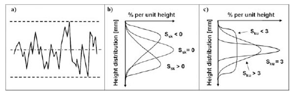). A surface with skewness above zero and kurtosis above three consists of more and/or higher peaks than valleys. Since the S_sk and S_ku parameters are calculated by using the surface height (η) to a power of 3 and 4, respectively (see Table 1), outliers in the surface topography will influence the parameters significantly. S_sk and S_ku are both moderately affected by the sampling interval [30].

Fig. (3) The amplitude parameters skewness (Ssk) and kurtosis (Sku) are defined from the amplitude distribution curve. (a) Shows the surface simplified to a profile and (b) and (c) show examples of different skewness and kurtosis values. For a Gaussian surface Ssk = 0 and Sku = 3.

3.1.4. Volume Parameters

The surface volume parameters are all defined from the Bearing Area Ratio of the surface (Fig. 4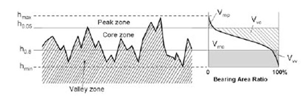). The parameters chosen were the material (V_mc) and void volume (V_vc) in the core zone together with the peak material (V_mp) and valley void volume (V_vv) of the bearing area curve of the topography. To calculate these parameters, the bearing area ratio is divided into peak, core and valley zones by horizontal lines parallel to the average line at 5% and 80% in the Bearing Area Ratio curve, respectively [30]. The parameters were chosen because of their ability to visualise changes in bearing at different levels of the surface. The bearing of the surface may be correlated with the biomechanical properties of the surface and the long term anchoring of the implant.

Fig. (4) Schematic description of the volume parameters defined from the bearing area ratio.

The S_a and S_q parameters are strongly correlated (see Table 1), which gives plots with the same appearance. Since the S_a parameter is more widely used in the dental implant literature, it was chosen to illustrate the dependence on filter size (Fig. 5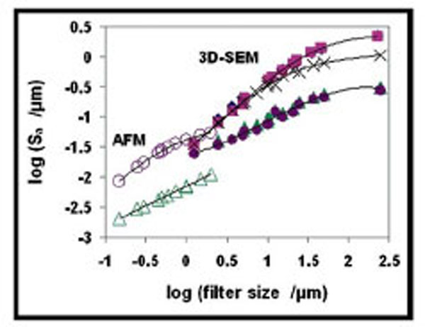). The S_a value increases with increasing filter size for all surfaces and the TS surface is well separated from the blasted surfaces over the entire filter size range. For filter sizes above 5 μm it is also possible to discriminate between the fine blasted (FB) and coarse blasted (CB) surfaces. The parameter values in this filter size range are obtained from all applied filter sizes in the ×500 3D-SEM magnifications and from the 10, 15, and 20% filter sizes in the ×1200 3D-SEM magnification.

Fig. (5) Log (Sa) as a function of log(filter size/μm) for all surfaces analysed. Values obtained from the 3D-SEM techniques are plotted as filled symbols while AFM results are shown as empty symbols. The lines are presented expressively to guide the eye. The unfiltered AFM data are encircled in the figure. ♦ = CB, ■ = CB+HF, × = FB, ▲ = TS, ● = TS+HF. Unfilled symbols represent AFM data.

With the S_a (or S_q) parameter it is not possible to observe changes due to the chemical treatment at any filter size or magnification (compare the curves for CB and CB+HF in Fig. (5)). However, differences between the two surfaces are clearly observed in the SEM images shown in Fig. (1). The fact that the calculated S_a value is unable to reveal the differences seen in the analogue image shows the limitation in digitalising the images. By using AFM, smaller surface features become accessible and a clear distinction between the TS and TS+HF surface is seen in the calculated S_a value (Fig. 5). The unfiltered values obtained from the 10×10 µm scan size in AFM fall on the same line as the values from 3D-SEM for the same surfaces. The values are encircled in Fig. (5). The HF etching clearly introduces changes in the surface topography at the sub-micrometre to nanometre level (see Fig. 1).

From the qualification tests made with the MeX^® software, the skewness (S_sk) parameter was shown to be affected by instrumental settings and large variations in S_sk were obtained for the same surface. Fig. (6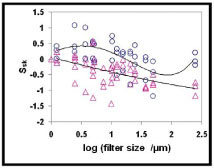) shows the S_sk parameter values for the CB and FB surfaces, where the rings and triangles are values from the three analysed spots and the line is the average of all obtained values. For the CB surface the S_sk values are around zero (Gaussian distribution) but changes from positive to negative values with increasing filter size. In contrast, the S_sk parameter is negative over the entire filtering range for the FB surface. A negative value for S_sk points at a surface with more and/or deeper valleys than peaks.

Fig. (6) Skewness (Ssk) values obtained for the coarse (○ = CB) and fine (∆ = FB) blasted surfaces by the 3D-SEM technique. Symbols represent single values obtained on all three analysed areas and the line represents the average.

The appearance of the kurtosis curve is similar to that of the skewness curve. Fig. (7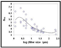) shows S_ku values obtained from all three spots on the CB surface. Also in this case a large spread in parameter values is observed. The S_ku value decreases from about 6 to 3.5 as the filter size is increased. For a Gaussian surface, the S_ku value is 3 and the larger values found for the CB surface show a peaky surface even though the S_sk values were grouped around zero indicating a Gaussian distribution. Although the variation in the S_ku parameter for the same surface was quite large for all surfaces, some trends could be seen. In Fig. (8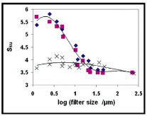) the S_ku values for all blasted surfaces are plotted together. The CB and CB+HF surfaces are overlapping with decrease in the S_ku with increased filter size. For the FB surface the S_ku parameter is independent of filter size with a value around 3.8. Thus, also for the FB surface some peakedness is observed. This is in agreement with the negative value of the skewness parameter since more and/or deeper valleys will lead to sharper peaks.

Fig. (7) Kurtosis (Sku) values for the coarse blasted surface (CB). Rings represent single values obtained on all three analysed areas and the line represents the average

Fig. (8) Average kurtosis (Sku) values (3D-SEM technique) for the blasted surfaces. The fine and coarse blasted surfaces are separated at lower filter sizes. No separation was obtained between the blasted and chemically treated surfaces. ♦ = CB, ■ = CB+HF, × = FB.

No change was observed after the chemical treatment of the turned and blasted surfaces probably due to the large spread in the S_sk and S_ku values. This also applies to the measurements with AFM.

Fig. (9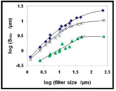) shows the S_10z average values for the CB, FB and TS surfaces. As expected, the lowest S_10z values were obtained for the TS surface followed by the FB and CB surfaces. With the S_10z parameter it is possible to discriminate between the fine and coarse blasted surfaces over the whole 3D-SEM range with slightly increased separation with increasing filter size. However, no change in the S_10z parameter was observed after the HF etching of the CB and TS surfaces using 3D-SEM, Fig. (10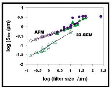). With the AFM technique a better resolution between the TS and TS+HF surfaces could be obtained. The values obtained by AFM and 3D-SEM are similar for the TS+HF surface but for the untreated TS surface the values obtained by the AFM technique are significantly lower. This is probably due to differences between the two techniques and will be further discussed in section 5.1.

Fig. (9) Average log(S10z) values for the fine and coarse blasted (FB and CB) surfaces together with the turned surface (TS). Separation is achieved between all three surfaces over the whole SEM range. ♦ = CB, × = FB, ▲ = TS.

Fig. (10) Average log(S10z) values for the turned surfaces with and without HF treatment. No separation is achieved within the SEM range whereas higher values are obtained for the etched surface within the AFM range. ▲ = TS, ● = TS+HF. Unfilled symbols represent AFM data.

Fig. (11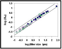) shows the autocorrelation length parameter, S_al, for the TS and TS+HF surfaces over the entire filter size range including both AFM and 3D-SEM measurements. A linear relationship is observed for all surfaces with a slope close to one, i.e. S_al is directly proportional to the filter size. This illustrates that the frequency of the measured roughness is defined by specifying the filter size, i.e the surface roughness is self-affined. Thus, it is important to measure surface roughness parameters as a function of filter size to fully describe the surface.

Fig. (11) Average log(Sal) values for all surfaces and both techniques. The slope of the line is close to one. ▲ = TS, ● = TS+HF. Unfilled symbols represent AFM data.

The S_tr parameter gives information about directional texture or randomness of the surface [28, 30]. A value below 0.3 indicates the presence of a directional texture while a value above 0.5 indicates a random surface structure. Fig. (12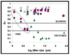) shows the S_tr values for the turned and blasted surfaces. The coarse blasted (CB) surface shows a transition to directional texture at the largest magnifications. The opposite is seen for the turned surface (TS) which shows directional texture for the larger filter sizes (low magnification) but approaches a more random surface structure at the smaller filter sizes. A small effect of chemical treatment was observed at the largest magnifications; see the encircled area in Fig. (12). In order to explain these results, the plots are evaluated together with SEM and AFM images.

Fig. (12) Average texture aspect ratio (Str) for the FB, CB, CB+HF and TS surfaces. Randomness is obtained for the FB surface over the whole SEM range while texture can be seen for the CB and CB+HF surfaces at the highest magnification (lowest filter sizes). The turned surface is classified as textured surface at the higher filter sizes and goes towards a random structure at the lower filter sizes. ♦ = CB, ■ = CB+HF, × = FB, ▲ = TS.

In Fig. (13) the SEM images for the FB and CB surfaces are compared. Three different magnifications are used together with three filter sizes in order to cover the whole 3D-SEM filter size range. For both surfaces the S_tr values are above 0.5 in the lower magnification region and were identified as random structure (Fig. 12). However, at the highest magnifications, texture was found for the CB surface but not for the FB surface. Blasting with larger particle size creates surface features of larger size, which can be seen at the higher magnifications in the SEM images in Fig. (13). The larger features may still have unaffected parts with a reminiscence from the turned surface. Another possible explanation is that at high magnifications only few surface features are analysed on the CB surface which can give an apparent directional texture. For the FB surface the features created are smaller and turning tracks are thus completely destroyed leading to a random surface also at the highest magnifications. Furthermore, the greater number of surface features reduces the probability of obtaining a false directional pattern. For the coarse blasted and chemically etched surface (CB+HF) the small features created somewhat masks the turning tracks and the surface is less textured. As expected, the TS surface is textured at large filter sizes due to the turning tracks on the surface. This is clearly seen in the SEM images in Fig. (14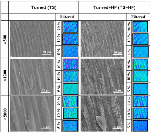). When filter sizes are decreased, the turning tracks disappear which explains the increase in S_tr value at the highest magnification, see the 5% filter size for the two largest magnifications.

Fig. (13) The FB and CB surfaces at three different SEM magnifications together with filtered MeX® images after application of filter with sizes 20%, 10%, and 5% of the horizontal image width. The depth scale of the MeX® filter images goes from purple which represents the deepest, through blue, green, and yellow up to red which represents the highest points on the surface. The depths are all different in the images. As seen in the filtered images, the fine blasted surface (FB) consists of smaller surface features than the coarse blasted surface (CB).

Fig. (14) SEM images collected at three different magnifications for the turned surfaces with and without HF treatment (TS and TS+HF) together with filtered MeX® images after application of filter with sizes 20%, 10%, and 5% of the horizontal image width. Differences between the two surfaces become more visible with increased magnification. The MeX® filtered images show quite clearly that the turning tracks are erased more and more by the application of smaller filter sizes.

Fig. (15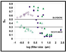) shows the S_tr parameter for the TS and TS+HF surfaces for both 3D-SEM and AFM. In the AFM analysis the S_tr values for the two surfaces are well separated, clearly showing the effect of the HF etching. In the 3D-SEM analysis similar S_tr values are obtained for the two surfaces with a clear texture at large filter sizes and an apparent random surface when the filter size is decreased. Since AFM has a higher resolution the difference in the values obtained with the two techniques shows the limitation of the 3D-SEM technique at the larger magnifications. In AFM the TS surface is textured in the entire filter size range while the TS+HF surface is random. This is also clearly seen in the AFM images shown in Fig. (16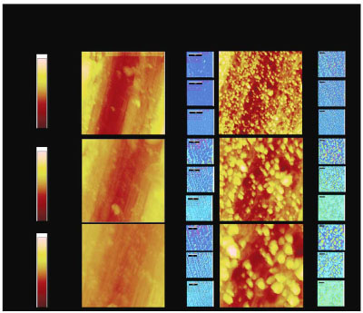). For the TS surface the turning tracks are observed also at the highest magnification and smaller filter size (3×3 μm, 5%). The small features created in the chemical pre-treatment are clearly seen in the AFM images and these precipitates effectively mask the turning tracks and the surface appears random.

Fig. (15) Average Str parameter values for the turned surfaces with and without HF treatment for both characterisation techniques. Both surfaces go from random to textured surfaces with increased filter size within the SEM range. For the AFM range, the chemically etched surface is classified as a random surface over the whole range while the untreated surface goes from the mixed zone to textured surface with increased filter size. ▲ = TS, ● = TS+HF. Unfilled symbols represent AFM data.

Fig. (16) AFM images collected at the three different scan sizes of the turned surface with and without HF treatment (TS and TS+HF), together with filtered MeX® images after application of filter of sizes 20%, 10%, and 5% of the horizontal image width. The chemical treatment induces a topography consisting of small peaks which covers the surface. By application of filters, the turning tracks are erased and a very smooth surface is created for the turned surface (TS).

The hybrid parameters are significantly affected by the sampling interval [30] which is changed with magnification and scan size of the SEM and AFM technique. This results in changes in absolute parameter values but the trend for the different surfaces is the same. This is showed by the S_dr parameter at ×500 magnification 3D in Fig. (17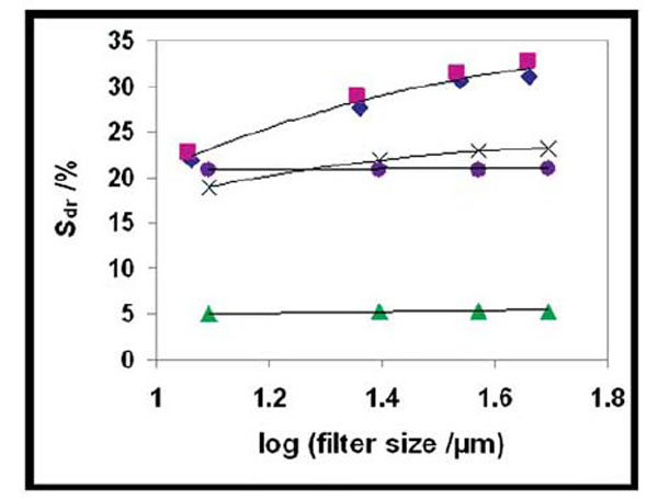). For the blasted surfaces S_dr increases with increasing filter size while smaller changes are observed for the turned surface. There is a clear difference between the TS, FB and CB surfaces with high values for the blasted surfaces and a much lower value for the turned surface. The HF etching increases the S_dr value slightly for the blasted sample but has a profound influence on the value for the turned surface (Fig. 17). Note that after the chemical treatment of the turned surface the S_dr values are similar to those of the fine blasted surface. Preliminary results show that the S_dq parameter can be used to estimate the interface shear strength [37] and it is therefore important to include this parameter in characterising surface roughness.

Fig. (17) Average log(Sdr) values for all surfaces at the lowest SEM magnification (×500). A similar relationship was obtained for the Sdq parameter. ♦ = CB, ■ = CB+HF, × = FB, ▲ = TS, ● = TS+HF. Unfilled symbols represent AFM data.

The results obtained for the S_dr and S_dq parameters actually indicate that changes on very small levels can be recorded in the 3D-SEM method. This is an important finding and will be further discussed in section 5.2.

All volume parameters show the same dependence on filter size for all surfaces and the relationship between the surfaces is similar to the relationship seen for the S_a and S_q parameters. For visualisation, the V_vc (void volume in core material) was chosen and is presented in Fig. (18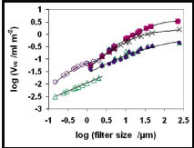). The values for the V_vc are well separated for the TS, FB and CB surfaces. For the latter two, similar values are obtained for filter sizes less than 5 μm which is similar to the findings for the S_a parameter. The V_vc is not affected by HF etching on coarse blasted and turned surfaces in the 3D-SEM filter size range. However, in AFM a clear difference in the V_vc values is observed after HF etching of the turned surface (Fig. 18). Unfiltered data at 10×10 μm scan size for both surfaces are in the same range as the data obtained with comparable filter size in the 3D-SEM technique (data encircled in Fig. (18)).

Fig. (18) Average log(Vvc) values for all surfaces obtained using AFM and 3D-SEM. Similar relationships were obtained for all volume parameters. ♦ = CB, ■ = CB+HF, × = FB, ▲ = TS, ● = TS+HF. Unfilled symbols represent AFM data.

In Table 2 an overview of the surface roughness parameters ability to discriminate between the different surfaces is given. By the 3D-SEM technique, the fine-, and coarse blasted surfaces were separated at the larger filter sizes in ten of the thirteen parameters evaluated (denoted as Partly in Table 2). With these ten parameters, the turned surface was well separated from the blasted surfaces in the entire filter size range. By the AFM technique the TS and TS+HF surfaces were well separated by ten of the evaluated parameters, while with the 3D-SEM technique it was not possible to separate the chemically treated and untreated surfaces (Table 2).

Table 2

Overview of the Surface Roughness Parameters Ability to Discriminate Between the Analysed Surfaces

For most of the parameters, differences between values calculated from the AFM and 3D-SEM techniques are observed (Figs. 5, 10, 15). The different values obtained may originate from a difference in the size of the area analysed, reflected in the filter size, or differences in the measurement techniques [34]. In 3D-SEM, a grey-scaled image is obtained by electron bombardment and converted to a matrix of data points used for calculating the surface roughness parameters. The AFM technique is a scanning probe technique where a probe is mechanically scanned over the surface and topographical height information is obtained from the force between the tip and the surface. In AFM the sensitivity is dependent on the tip size in relation to the roughness and in 3D- SEM the limiting factors are the quality of the image and the resolution.

In this study, the SEM images and AFM data were imported into the MeX^® software where parameters were calculated. The pixel distance used in the SEM image or AFM scan gives the lowest resolution limit possible of the images in the MeX^® software. Although the pixel distance for SEM ×2500 and ×5000 images and AFM 10×10 μm and 5×5 μm scan sizes are similar, it was not possible to distinguish between the TS and TS+HF surfaces using 3D-SEM together with the MeX^® software. This shows that the small surface features induced by the chemical etching are below the detection limit for 3D-SEM. The resolution limit for 3D-SEM together with the MeX^® software could be affected by various parameters such as: brightness and contrast of the images, disturbances from outside vibrations not allowing for sufficient magnification or resulting in blurry images, imperfectly overlapping stereo-SEM pair resulting in loss of sharpness of the 3D-models and shadowing effects masking some parts of the area. In the qualification of the method, the effect of brightness and contrast on the calculated roughness parameters was evaluated and only if very bright or dark images were collected an effect on the parameters was obtained. Blurry images will give a contribution to the parameter values related to the height resolution for different magnifications and filter sizes.

The hybrid parameters, S_dr and S_dq, were the only parameters able to distinguish between the turned and etched (TS and TS+HF) surfaces within the 3D-SEM range (Table 2 and Fig. 17). These parameters are combinations of amplitude and spatial characteristics of the surface [28]. With S_dq for example, the derivative with respect to the surface height is obtained, which is more sensitive to changes at all levels than the amplitude parameters S_q or S_a. Since none of the amplitude or spatial parameters alone were able to distinguish between the TS and TS+HF surface, this shows that parameters from all groups (amplitude, spatial and hybrid) need to be used to be able to distinguish between different surfaces.

Low values for both evaluated hybrid parameters were obtained for the turned surface (TS) compared with the etched surface (TS+HF) showing the peakedness introduced by the etching. It is interesting to note that the TS+HF surface has similar S_dr and S_dq values as the fine blasted (FB) surface by the 3D-SEM technique (Fig. 17). The FB surface consists of higher surface features than the TS+HF surface, increasing the S_dr and S_dq value according to the equations shown in Table 1. However, the S_dr and S_dq parameters are also affected by the number of surface features present and captured by each pixel of the analysed surface. Since the TS+HF surface consists of a larger number of surface features, this will contribute to the S_dr and S_dq values. This explains the similar values for both the TS+HF and FB surfaces.

When comparing the two analysing techniques, higher S_dr values for the TS+HF surface were obtained by AFM compared with 3D-SEM, 3% and 55% (AFM 10×10 μm), 5.5% and 20.6% (3D-SEM ×500), for the TS and TS+HF surfaces, respectively. Also higher S_dq values were recorded with AFM. Both S_dr and S_dq parameters are sensitive to the pixel distance (i.e. sampling interval [30]) since a larger pixel distance works as a smoothing of the surface. In general AFM is therefore more sensitive than the 3D-SEM technique with smaller analysing area and pixel distances. However, in the present study comparable pixel distances were obtained in a few cases but the differences remained; see section 5.1 for further discussion.

For engineering applications functional parameters are commonly defined to describe certain properties related to wear, bearing etc. [29, 30]. The functional parameters are given in terms of the average height parameter, S_q, to eliminate the effect of roughness and highlight other surface properties. For characterising dental implants the fluid retention index, S_ci, has been used [3, 31]. S_ci can be calculated by Equation 1[29] and describes the ability of the surface to keep the fluid. This is important for tribology and might also be important for the tissue-implant contact.

The S_ci parameter for the surfaces analysed in the present study was calculated and found to be between 1.1 and 1.3. This value is independent of the technique used and of magnification and filter size. For a Gaussian surface, S_ci is 1.56 and for sand blasted and turned surfaces the S_ci values are commonly around this value or higher. The low value obtained in the present study is probably an effect of the placement of the reference plane. As previously described, the reference plane was placed on the most even parts of the surface and for plateau type surfaces the S_ci value is much lower [29].

In two recent studies, the retention strength in vivo was correlated to the S_ci index [3, 31]. Inconsistent results were reported with increased retention strength for surfaces with high [3] and low [31] S_ci index, respectively. Arvidsson et al. [31] compared different blasted surfaces as well as the surfaces of a number of commercially available implants. The S_ci index for all these surfaces, except TiUnite, is very similar ranging from 1.36 to 1.57 including the turned surface as a reference. For TiUnite the S_ci value falls outside this range with S_ci = 1.86. Since different surfaces give the same S_ci value it is questionable to correlate the S_ci index to the in vivo performance. A better choice would be the volume parameter alone since for dental implants the entire surface is important for the in vivo performance. The volume property of a surface is known to be important when two surfaces are in close contact, for example during wear and bearing situations [29, 30]. In the in vivo situation, the bone and implant are in close contact and the surface topography is known to affect the retention forces measured in vivo [9-16]. A correlation with volume parameters may therefore exist and will be discussed in Section 5.5.

Surface roughness parameters are in general scale-dependent and it is therefore important to perform a variable length scale analysis. For implant surfaces this scale dependence is of prime interest since roughness at different levels may contribute to the performance in vivo. For example, the physical surface treatment by blasting introduces roughness on the micrometer level and contributes to a better anchoring of the implant while chemical modifications give roughness on a smaller length scale. The fact that surfaces with the same blasting treatment but different chemical treatment show differences in performance clearly demonstrates that the finer topography introduced by the chemical treatment is important. This effect acts in parallel with any direct chemical influence introduced by changes in the surface composition or changes in the titanium dioxide properties [41]. Different methods have been proposed to accommodate the length scale dependence of surface roughness parameters including wavelet filtering, fractal analysis [34, 42-48] and Fast Fourier Transform [22, 23]. Variable length scale analysis is applicable both to fractal and non-fractal surfaces and the fractal dimension of a surface is commonly evaluated if applicable. The analysis is based on a log-log plot of a characteristic roughness parameter versus a length scale defined as the filter size in the present work. Many natural and man-made surfaces have fractal character at least over part of the length scale and fractal analysis, being a scale independent method, has been extensively used to characterise engineering surfaces [42, 45, 48, 49]. A fractal surface can be described by a power law, exemplified here by the surface roughness parameter S_a and the filter size, Equation (2):

In the linear part of the log(S_a)-log(filter size) plot the surface can be represented by a self-affined fractal, characterised by the fractal dimension D. From the slope of the log-log plot the fractal dimension can be calculated according to Equation (3) [42]:

The fractal dimension is independent of filtering and has a non-integer dimension ranging from 2 for a completely flat surface to 3 representing a volume. Machined surfaces produced by more than one finishing process may have different fractal properties. The transition between two linear regions is defined by the crossover size, below which the surface is most simply described by fractal geometry. The crossover size together with the slope yields a more accurate description of the surface than either separately and has been used in the present analysis.

In the present work the changes in scale were accomplished by measuring at different magnifications and different filtering sizes. The filter size is defined in relation to the horizontal axis giving some overlap between different magnifications. For the amplitude and volume parameters in Figs. (5, 9, 10, 18), linear log-log relationships exist in certain filter size ranges and the fractal dimension was calculated using Equation (3). The crossover size was obtained from the crossover between the fractal behaviour (linear log-log plot) and the saturation roughness at the smallest magnification. For the TS surface, no crossover could be defined showing that for both 3D-SEM and AFM the TS surface can be represented by a self-affined fractal in the whole filter size range. In Table 3, the fractal dimensions for the different surfaces are given together with the crossover sizes. These data are based on the S_a values but similar values are obtained when analysing the other parameters.

Table 3

Fractal Dimension and Crossover Size Determined for the Studied Surfaces

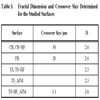
For the blasted surfaces the fractal dimension was 2.6 with a crossover of 30 µm for the coarse blasted surfaces and 20 µm for the fine blasted surface. The fractal dimension for the turned surface was 2.3. The chemical etching with HF did not influence the fractal dimension for the blasted and turned surface examined by 3D-SEM. However, a clear difference is observed in AFM for the TS+HF surface. The fractal dimension is the same as for the blasted surfaces but the crossover size is much smaller, 1.1 µm, showing the level of roughness. The fact that the fractal dimension for the TS+HF surface is similar to the values obtained for the FB surface is in accordance with the S_dr (S_dq) values (Fig. 17). Comparing the crossover size with the AFM images in Fig. (16) reveals that the surface features are smaller than the crossover size. The fine structure in the low micron or nanometer range is often hidden by coarser contributions to the roughness and for the 3D-SEM technique the smallest features were not at all detectable, i.e. no change in the fractal dimension for the TS+HF surface and no crossover.

In order to understand the differences observed for the two techniques used, model surfaces were analysed. Fig. (19a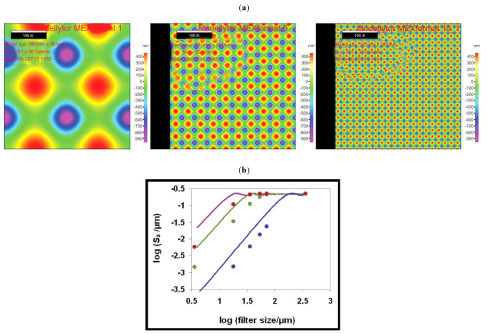) shows the three surfaces used with different density of features on the surface. The data were analysed in MeX^® in the same way as the experimental surfaces and by an alternative way originating from fractal analysis, denoted “power law analyses” below. In the latter case the area of analysis was continuously decreased from the full size down to a few pixels and the S_a-values were plotted as a function of the number of pixels (N) on the horizontal axis in a log-log plot (Fig. 19b). The change in area was made in such a way that the same ratio between the horizontal and vertical axes was maintained. Since the same function is used to generate the different surfaces and only the number of surface features differs, the S_a value should be the same provided that enough features are present. Fig. (19b) clearly shows that this is the case. The S_a value is oscillating around a constant value showing the corrugation of the surface down to a certain number of pixels defined by the size of the surface features in relation to the pixel size. At lower values of N, log(S_a) is linearly related to log(N) with a slope close to two for these model surfaces, i.e. a fractal dimension close to three. The crossover between the constant and linear parts defines the smallest surface feature that can be detected. Consequently, the crossover point moves to lower log(N) values as the number of surface features increases, i.e. gets smaller. In Fig. (19b) the data from the MeX^® analysis are also plotted and the same general trend is observed. However, the crossover is larger compared with the power law analysis. In the power law analysis used in the present work the smallest area is located in the centre of the image and has the form of a cone. The linear part of the log-log plot corresponds to diminishing height of the cone and the crossover is the upper size of the cone. The fractal dimension is close to 3 since the volume of the cone is analysed at the smallest length scale. In the MeX^® analyses the filtering smears out the surface features somewhat and the crossover is larger than expected theoretically. This is the same behaviour as observed for the experimental surfaces and shows the limitation of the MeX^® analyses. A better resolution of the fine structure can be obtained by variable length analyses as shown for the model surfaces. However, in order to get better statistical values the surface roughness parameters should be calculated over the entire surface using different sizes of the analysing area in a similar way as described in Chauvy et al. [34]. This approach will be explored in a forthcoming paper.

Fig. (19) (a) Model surfaces with 4, 100 and 400 protruding surface features, respectively, and (b) log(Sa) as a function of log(N). The symbols are from the MeX® analysis and the lines from the power law analysis.

The main goal for characterising implant surfaces in great detail is to obtain a relationship between surface roughness parameters and the performance of the implants in vivo. Such a relationship would be beneficial for the development of new surfaces and would also minimize the need for animal studies. The relationship between in vivo results and surface roughness parameters such as S_a has been previously emphasised [16, 32, 50, 51] but as described in Section 5.3 for example the fluid retention index seems to give contradictory correlation results. If we assume that the volume parameter used to calculate the fluid retention index is a better predictor of the in vivo performance then a correlation between this parameter and for example the removal torque (RTQ) value should exist. However, since volume parameters are very rarely given in the literature such a relationship will be difficult to prove. Since the volume parameters show the same general behaviour with filter size as the S_a parameter, compare Figs. (5) and (18), the S_a value can be used instead. Literature values from in vivo tests performed in rabbit, were collected for implant surfaces similar to the surfaces studied in the present paper [12, 52-54]. In Fig. (20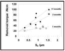), removal torque data are plotted as a function of S_a. The data are collected from different sources and it may be questioned if a comparison is at all feasible. However, Fig. (20) clearly shows a linear relationship between removal torque and the surface roughness parameter S_a, with increasing removal torque values for surfaces with higher S_a value. This applies both to data obtained after 1 and 3 months. Extrapolation to S_a = 0, i.e. a surface without roughness, gives the same removal torque value for both 1 and 3 months test. This fact was used to get the relationship between removal torque and S_a for the few data found for 12 months test.

Fig. (20) Removal torque values on rabbit after one, three and 12 months. The surfaces studied were TS [12], FB [12, 52, 53], FB + HF [53], CB [54] and CB + HF [52, 54].

The removal torque data obtained after one month falls on a line and the HF treatment has minor additional effect on the removal torque after a short implantation time. One value for the FB surface falls outside the linear range [12] showing the same removal torque value after 3 weeks and 3 months. Also after 3 months, RTQ increases with increasing S_a value for all surfaces except the fine blasted surface with HF etching [53], which shows a much higher removal torque value than expected. The reason for the high value is not known. However, in one study comparing the RTQ between coarse blasted surfaces with and without HF treatment increased RTQ was indeed found for the HF treated surface [54]. In addition, Ellingsen et al. [55] have shown improved bone-to-implant attachment for coarse blasted surfaces treated with hydrofluoric acid using pull-out experiments and in a recent study the semiconducting properties of the oxide were related to the enhanced performance [41]. Note that the data reported in Fig. (20) are restricted to turned and blasted surfaces with and without chemical etching with HF. Thus, for this restricted set of surfaces there is a clear relationship between the S_a parameter and the removal torque value. This implies that ways of increasing S_a for blasted surfaces, such as chemical etching and deposition, will give better anchoring results in vivo.

In order to look for some generality in the correlation between S_a and removal torque other surfaces were also analysed. For aluminium oxide blasted surfaces [56] the removal torque values are lower compared with the TiO₂ blasted surfaces but the general trend is the same, i.e. the removal torque value increases with increasing S_a value. The presence of Bonit^® (calcium phosphate) on the surface seems not to further increase the removal torque value indicating that the geometrical changes are dominating the in vivo performance. On the other hand, in the presence of hydroxyl apatite (HA) on fine blasted surfaces (FB) [12] the removal torque value after 3 and 12 weeks are much higher than expected from the relationship shown in Fig. (20).

A set of anodized surfaces have been subjected to an in vivo study measuring the removal torques values after 6 weeks [57]. Anodising to different potential results in a thicker titanium oxide layer but the S_a value is only slightly increased. The removal torque values are fairly constant and little additional effect of the anodisation is observed.

In addition to the increase in surface roughness, there might also be a chemical stimulation as observed for hydroxyl apatite [12] and HF etching [53, 54]. Another example is inclusion of magnesium. In most cases the inclusion of Mg by oxidation of the titanium surface results in significantly higher removal torque values compared with changes in the surface roughness [12, 58, 59]. This illustrates that by a general comparison between surface roughness and in vivo results it is also possible to discriminate between a purely geometrical effect, a chemical effect, or a combination of both for the improved in vivo performance.