- Home
- About Journals
-
Information for Authors/ReviewersEditorial Policies
Publication Fee
Publication Cycle - Process Flowchart
Online Manuscript Submission and Tracking System
Publishing Ethics and Rectitude
Authorship
Author Benefits
Reviewer Guidelines
Guest Editor Guidelines
Peer Review Workflow
Quick Track Option
Copyediting Services
Bentham Open Membership
Bentham Open Advisory Board
Archiving Policies
Fabricating and Stating False Information
Post Publication Discussions and Corrections
Editorial Management
Advertise With Us
Funding Agencies
Rate List
Kudos
General FAQs
Special Fee Waivers and Discounts
- Contact
- Help
- About Us
- Search


The Open Mechanical Engineering Journal
(Discontinued)
ISSN: 1874-155X ― Volume 14, 2020
The Dynamics of One Way Coupling in a System of Nonlinear Mathieu Equations
Alexander Bernstein1, Richard Rand2, *, Robert Meller3
Abstract
Background:
This paper extends earlier research on the dynamics of two coupled Mathieu equations by introducing nonlinear terms and focusing on the effect of one-way coupling. The studied system of n equations models the motion of a train of n particle bunches in a circular particle accelerator.
Objective:
The goal is to determine (a) the system parameters which correspond to bounded motion, and (b) the resulting amplitudes of vibration for parameters in (a).
Method:
We start the investigation by examining two coupled equations and then generalize the results to any number of coupled equations. We use a perturbation method to obtain a slow flow and calculate its nontrivial fixed points to determine steady state oscillations.
Results:
The perturbation method reveals the existence of an upper bound on the amplitude of steady state oscillations.
Conclusion:
The model predicts how many bunches may be included in a train before instability occurs.
Article Information

Identifiers and Pagination:
Year: 2018Volume: 12
First Page: 108
Last Page: 123
Publisher Id: TOMEJ-12-108
DOI: 10.2174/1874155X01812010108
Article History:
Received Date: 20/12/2017Revision Received Date: 21/03/2018
Acceptance Date: 04/04/2018
Electronic publication date: 30/04/2018
Collection year: 2018
open-access license: This is an open access article distributed under the terms of the Creative Commons Attribution 4.0 International Public License (CC-BY 4.0), a copy of which is available at: (https://creativecommons.org/licenses/by/4.0/legalcode). This license permits unrestricted use, distribution, and reproduction in any medium, provided the original author and source are credited.
* Address correspondence to this authors at the Dept. of Mathematics, Cornell University, Ithaca, NY 14850, USA; Tel: 607 255 8198; E-mails: rhr2@cornell.edu, rrand1@twcny.rr.com
| Open Peer Review Details | |||
|---|---|---|---|
| Manuscript submitted on 20-12-2017 |
Original Manuscript | The Dynamics of One Way Coupling in a System of Nonlinear Mathieu Equations | |
1. INTRODUCTION
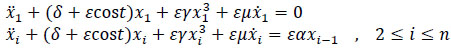
In this paper, we investigate the dynamics of the following system of n nonlinear Mathieu equations:
 |
(1) |
 |
(2) |
The Mathieu equation is a Hill equation with only one harmonic mode and is an example of parametric excitation. Parametric excitation has been well studied in general [1J. Cuevas, L.Q. English, P.G. Kevrekidis, and M. Anderson, "Discrete breathers in a forced-damped array of coupled pendula: Modeling, computation, and experiment", Phys. Rev. Lett., vol. 102, no. 22, p. 224101.
[http://dx.doi.org/10.1103/PhysRevLett.102.224101] [PMID: 19658866] -2M. Syafwan, H. Susanto, and S.M. Cox, "Discrete solitons in electromechanical resonators", Phys. Rev. E Stat. Nonlin. Soft Matter Phys., vol. 81, no. 2 Pt 2, p. 026207.
[http://dx.doi.org/10.1103/PhysRevE.81.026207] [PMID: 20365638] ], and the Mathieu equation has been well studied in particular [3C.S. Hsu, "On a restricted class of coupled Hill’s equations and some applications", J. Appl. Mech., vol. 28, no. 4, pp. 551-556.
[http://dx.doi.org/10.1115/1.3641781] -5I. Kovacic, R.H. Rand, and S.M. Sah, "Mathieu’s equation and its generalizations: Overview of stability charts and their features", Appl. Mech. Rev., vol. 70, no. 2, p. 020802.
[http://dx.doi.org/10.1115/1.4039144] ]. One of its most salient features is that it has an infinite number of tongues of instability that grow out of the points  in the δ - ε plane, where n is an integer. As n gets larger, the size of each tongue gets narrower, and so the most significant tongue is the one at
  . This tongue corresponds to a 2:1 subharmonic resonance, and shall be the focus of this paper.
The effect of nonlinearity is to limit the growth of trajectories around the instability; instead of trajectories spiraling towards infinity, they tend towards a stable limit cycle. Of particular interest here is the amplitude of the limit cycle and how that amplitude depends on the various parameters in the problem.
We will investigate the effect of one-way coupling on nonlinear Mathieu equations in this paper. In particular, we will demonstrate that when the amplitude of the coupling coefficient, α, is small enough, the coupled oscillators (2) can have multiple steady state oscillations, and one of these is smaller than the steady state of the uncoupled oscillator (1). When α is large enough, there is only one possible steady state oscillation. In all cases, the sizes of the limit cycles are bound by an upper bound.
It should be noted that this work is based on the assumption that the forcing frequency is constant. The case where the forcing frequency changes as the system spins up has been treated in a recent paper [6G.M. Wang, T. Shaftan, V. Smaluk, Y. Li, and R. Rand, "Lossless crossing of a resonance stopband during tune modulation by synchrotron oscillations", New J. Phys., vol. 19, no. 9, p. 093010.
[http://dx.doi.org/10.1088/1367-2630/aa8742] ] where it was shown that the system can pass through a resonance tongue without excessive growth if the passage is reasonably fast and the tongue is sufficiently narrow.
Our interest in Eqs.(1, 2) comes from an application in the design of particle accelerators.
1.1. Application
This work was motivated by a novel application in particle physics, namely the dynamics of a generic circular particle accelerator. Since this application is expected to be unfamiliar to most readers of this journal, we offer the following description of a synchrotron [7"Cornell Electron Storage Ring", CLASSE: CESR. Cornell laboratory for accelerator-based sciences and education, . Available from: http://www.lepp.cornell.edu/Research/CESR/WebHome.html].
The synchrotron is a particle accelerator in which a “Particle” actually consists of a group of electrons called a “Bunch,” and the collection of all bunches is called a “Train.” We ignore the interactions of electrons inside each bunch and treat the entire bunch as a single particle.
Each bunch leaves an electrical disturbance behind it as it traverses around the synchrotron, and these wake fields are the main source of coupling in the model. The coupling is mediated by several sources, including ion coupling and the electron cloud effect.
Particle paths in the synchrotron are circle-like but are not exact circles. Since the synchrotron lacks a central force, the circle-like particle orbits are achieved through the use of about 100 electromagnets spread around the periphery Fig. (1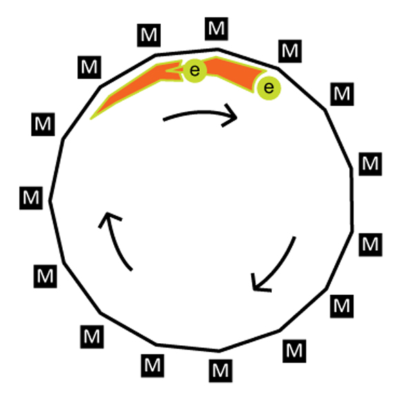 ).
).
 |
Fig. (1) Two bunches moving clockwise along a polygonal path through the use of a system of electromagnets. |
This means that the magnetic external forcing is periodic in rotation angle θ; assuming that the angular velocity of the bunch is constant with θ = ωt, the forcing is periodic in time as well. We can express this forcing function as a Fourier series, and we shall approximate this series by the first couple of terms in it, namely the constant term and the first cosine term.
We model each bunch as a scalar variable xi(t), i = 1,...,n. Here, xi is the vertical displacement above equilibrium of the center of mass of the ith bunch. Each xi is modeled as a damped parametrically-forced oscillator, and we write:
 |
The nonlinear terms are included to create a more realistic model since most natural phenomena are nonlinear and linear models are a convenient approximation. The nonlinear parameter, γ, can be chosen to adjust the scale of the problem.
The damping terms are also included to create a more realistic model.
The coupling terms on the right-hand side may be viewed as the strength of the plasma interactions: the radiation from a bunch produces an electron cloud which travels behind the bunch. This radiation dissipates away very quickly though, and so this coupling has a short range and can only influence the dynamics of the next bunch in the train. The coupling strength is affected by both the spacing between bunches as well as the charge of each bunch, and α encapsulates both of those effects.
2. TWO-VARIABLE EXPANSION
We use the two-variable expansion method [8J. Kevorkian, and J.D. Cole, Perturbation methods in applied mathematics.Applied Mathematical Sciences., vol. 34, Springer: Waltham, MA, ., 9R.H. Rand, Lecture Notes in Nonlinear Vibrations., Published on-line by The Internet-First University Press, . Available from: http://ecommons.library.cornell.edu/handle/1813/28989] to study the dynamics of Eqs. (1, 2). We set
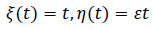 |
where ξ is the time t and η is the slow time.
Since the xi terms are functions of ξ and η, the derivative with respect to time t is expressed through the chain rule:
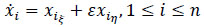 |
Similarly, for the second derivative we obtain:
 |
In this paper, we only perturb up to O(ε), and so we will ignore the ε2 terms.
We then expand the xi terms in a power series in ε:
 |
(3) |
In addition, we detune off the 2:1 subharmonic resonance by setting:
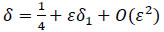 |
(4) |
Substituting ((3)), ((4)) into ((1)), ((2)) and collecting terms in ε, we arrive at the following equations:
 |
(5) |
 |
(6) |
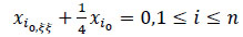
The solution to (5) is simply:
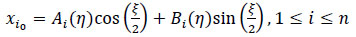 |
(7) |
We then substitute (7) into (6). Using trigonometric identities, these equations can be written in terms of  and
and  . We set the coefficients of such terms equal to zero in order to remove the secular terms which cause resonance. This results in 2n equations in 2n unknowns:
 |
(8) |
 |
(9) |
 |
(10) |
 |
(11) |
These equations are known as the slow flow of the system and represent the envelope of the oscillatory motion of equations (1, 2). Finding the equilibrium points of the slow flow is analogous to finding simple harmonic motion with constant amplitude in the original system. In doing so, we will not only obtain information on the amplitude of these limit cycles but also information on where Hopf bifurcations occur in parameter space.
3. ANALYTIC RESULTS
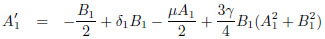
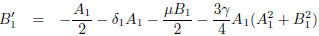
3.1. The First Bunch
The dynamics of the first bunch are given by eqs. (8, 9).
 |
As this system is 2-dimensional, the complete dynamics can be expressed in the phase plane A1-B1. The Numerical Results section contains various graphs demonstrating the full dynamics of the first bunch, but the rest of this section will focus purely on calculating the equilibrium points of the system.
Setting these equations equal to zero gives us the following equilibrium points:
 |
Here, we use the standard notation  to denote equilibrium points of the variables Ai, Bi.
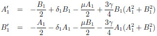
To simplify matters, we will focus on the special case when δ1 = 0 and μ = 0. Setting δ1 = 0 lets us examine the point of resonance directly without considering points in the neighborhood of the resonance, and setting μ = 0 ignores the effects of damping which ends up having a negligible effect on the analysis of the steady state. The fixed points in this case are:
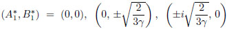 |
(12) |
Here, we note our first major observation: Nontrivial real equilibrium points for A1 only exist for γ < 0, and nontrivial real equilibrium points for B1 only exist for γ > 0. However, the magnitude of the amplitude is the same in both cases, and the analysis of both cases is identical. Without the loss of generality, we will take γ > 0 and  = 0.
= 0.
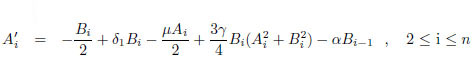
3.2. The Second Bunch
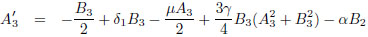
The dynamics of the second bunch are given when i = 2 in eqs. (10, 11).
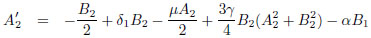 |
(13) |
 |
(14) |
Note that these equations share a similar structure to eqs. (8 and 9) but with additional terms resulting from the one-way coupling. These additional terms mean the dynamics of the second bunch are 4-dimensional instead of 2-dimensional like the first bunch, and we cannot view the dynamics in a phase plane. Our analysis of the second bunch will focus only on the steady-state solutions and not on the general dynamics.
Since we are taking γ > 0, all equilibrium points for the first bunch require = 0; substituting = 0 into eqs. (13, 14) yields:
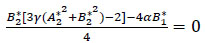 |
(15) |
 |
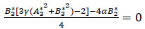
(16) |
Note that  +
+  is a nonnegative value, and is only identically zero in the trivial solution (, ) = (0,0). Since we are interested in nontrivial solutions, we require that + be positive.
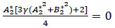
However, since γ > 0, the expression 3γ( + ) + 2 must be positive. Thus, the only way for (16) to equal zero is for  = 0.
= 0.
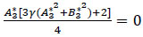
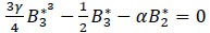
Substituting = 0 into (15) yields:
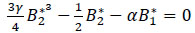 |
(17) |
Since  is already known to us from eq. (12), solving this cubic equation will give us the solution for
  .
.
This solution gives us the steady-state of B2. The full dynamics of the system is 4-dimensional, involving A1, B1, A2 and B2, and cannot be expressed in a phase plane.
A graph of the relationship between and α can be seen in Fig. (2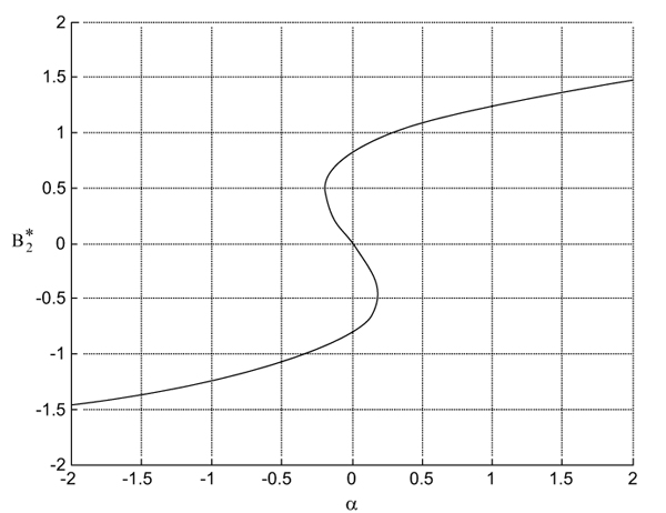 ).
).
3.3. The Third Bunch
The dynamics of the third bunch are given when i = 3 in eqs. (10, 11).
 |
(18) |
 |
(19) |
Note that these equations share the exact same structure as eqs. (13, 14). Just like with the second bunch, the presence of additional terms means that the dynamics of the third bunch are 4-dimensional. This means that we can’t view the dynamics in a phase plane, and so our analysis of the third bunch will focus only on the steady-state solutions and not on the general dynamics.
 |
Fig. (2) Plot of as a function of α, for γ = 1 and  . .
|
We know from the analysis of the second bunch that = 0 is necessary for all steady state solutions of the second bunch; substituting = 0 into eqs. (18, 19) yields:
 |
(20) |
 |
(21) |
Note that  +
+  is a nonnegative value, and is only identically zero in the trivial solution ( + ) = (0,0). Since, we are interested in nontrivial solutions, we require that + be positive.
However, since γ > 0, the expression 3γ( + ) + 2 must be positive. Thus, the only way for (21) to equal it to zero is for  .
.
Substituting into (20) yields:
 |
(22) |
Since is already known to us from eq. (17), solving this cubic equation will give us the solution for  .
.
The graph of the relationship between and α will look qualitatively similar to the relationship between and α Fig. (2) but they will differ quantitatively since the value of that is substituted into eq. (22) will in general be different than the value of that is substituted into eq. (17).
Still, given the similarity between eq. (22 and 17), it is natural to ask if this pattern continues for all later bunches. Indeed, this is the case, and so we will generalize the results found in these past two sections to the nth bunch in the system, where n can be any integer.
3.4. The nth Bunch
Due to the nature of one-way coupling, the dynamics of all the bunches except the first one are identical, as can be seen in the results found for the second and third bunches. Thus, we can easily derive a formula for calculating the steady-state solution for the nth bunch for any n > 1:
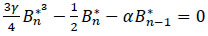 |
(23) |
Unfortunately, calculating  in practice requires calculating the amplitudes of all bunches in front of it, since the recursive relationship cannot be simplified into a formula dependent only on the first bunch. Part of the problem is that each step requires solving a cubic equation which, although solvable in principle, is a tangled mess. In practice, it is much easier to use numerical root solving methods to find the amplitudes for all the bunches.
The other, bigger problem is that cubic equations have three roots; if all three roots are real and distinct, then we have a multi-valued function. Fortunately, this only occurs for a range of α values, and we can easily determine this region through analytic means.
3.5. Multi-Valued Regions
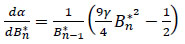
Note that in Fig. (2), there are two points with infinite slope: these are the points that divide the function into multi-valued regions and single-valued regions. If we flipped the two axes, then these two points change from having infinite slope to zero slopes see Fig. (3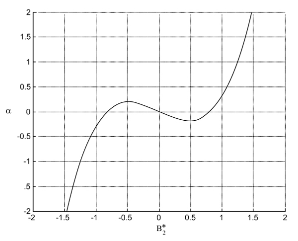 ). Thus, we want to derive
  and find the values of α for which the derivative is equal to zero.
 |
Fig. (3) Plot of α as a function of , for γ = 1 and .
|
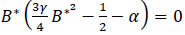
We start by moving the α term in eq. (23) to the right hand side and differentiating both sides.
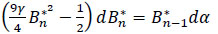 |
Here  is a constant since we’re assuming all
  up to i = n - 1 have already been found.
Solving for , we obtain:
 |
We set this equal to zero to find the local extrema:
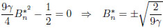 |
Finally, we substitute this result into eq. (23) to find the corresponding α value:
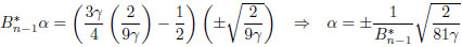 |
(24) |
One important feature of this result is that the range of α values for the nth bunch depends on the bunch before it. As an example, for , the α range depends on ; multiple limit cycles are possible for when α [-3-3/2,3-3/2] ≈ (-0.2,0.2).
The significance of this result is that fixing α does not guarantee that all bunches will be either multi-valued or single valued; it is possible to choose α such that only has one limit cycle, but has three.
A natural question to ask at this point is whether there exist values of α that do guarantee single valuedness for all . Due to the relationship of eq. (24), a uniform bound on α requires a uniform bound on , so this question is equivalent to asking if there is a bound on how large can become.
3.6. Limit as n → ∞
It turns out that the are indeed bound by an upper bound, and this can be shown by examining the limit as n → ∞.
In particular, we care about the limit of the amplitude ||. One way for this limit to exist is if B* = = as n → ∞. In this case, each bunch has the same amplitude as the bunch before it, and each bunch is oscillating in phase with the bunch before it.
By setting B* = = in eq. (23), we obtain:
 |
(25) |
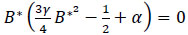
Thus, we find that the possible in-phase limits are:
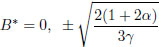 |
(26) |
As long as α ≥ - 1/2, these three limits are distinct; otherwise, no in-phase limit cycles are possible.
Another possibility is to examine the case when B* = = as n → ∞. In this case, each bunch has the same amplitude as the bunch before it, and each bunch is oscillating 180 degrees out of phase with the bunch before it.
By setting B* = = - in eq. (23), we obtain:
 |
(27) |
Thus, we find that the possible limits are:
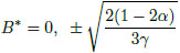 |
(28) |
As long as α ≤ 1/2, these three limits are distinct; otherwise, no out-of-phase limit cycles are possible.
Therefore, in the limit as n → ∞, there are three possible cases:
- For α < - 1/2, only out-of-phase limit cycles can exist.
- For -1/2 < α < 1/2, both out-of-phase and in-phase limit cycles can exist.
- For 1/2 < α, only in-phase limit cycles can exist.
- Fig. (4
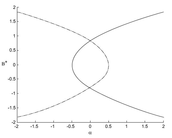 ) shows the upper bound for both types of limit cycles.
- Fig. (4
 |
Fig. (4) The solid curve is the upper bound on amplitude of the in-phase limit cycle. The dashed-dot curve is the upper bound on the amplitude of the out-of-phase limit cycle. |
4. NUMERICAL RESULTS
4.1. Phase Plane
To help visualize the dynamics of the first bunch, graphs showing the phase plane for eqs. (8 and 9) are provided below. All phase plane graphs were made using PPLANE [10 MATLAB v.7.5 by Mathworks; applet pplane7.m by Polking, J. C , Rice University, Department of Mathematics, Available from: http://math.rice.edu/∼dfield/dfpp.html].
Fig. (5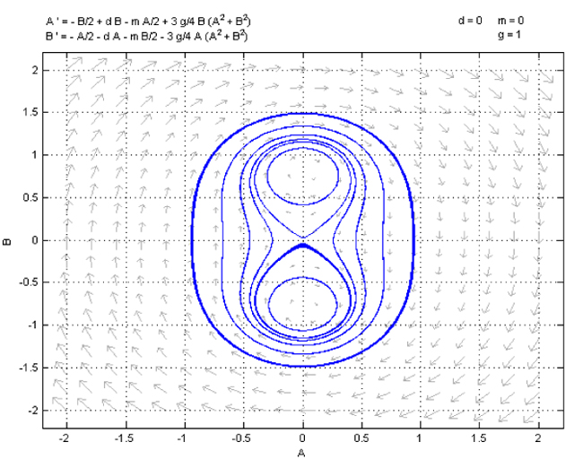 ) compares the cases when γ > 0 and γ < 0. Qualitatively, the graphs are the same; the only difference is that one has the equilibrium points on the A axis and the other has the equilibrium points on the B axis.
Fig. (6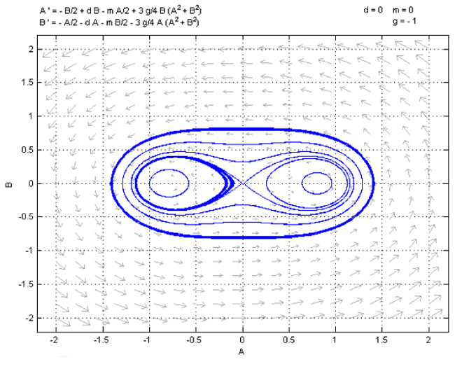 ) shows the effect of including small values of δ1 and μ. The inclusion of damping has broken the homoclinic orbit and all orbits are eventually attracted to one of the two stable equilibrium points. Since the two basins of attraction are intertwined, it can be hard in practice to determine which equilibrium point will be reached from a given initial condition.
Fig. (7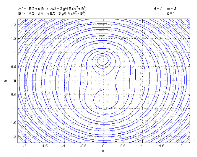 ) shows the effect of including larger values of δ1 and μ. The equilibrium points have gone through a pitchfork bifurcation and there is now only one equilibrium point: the origin.
4.2. Cobweb Diagram
Since all bunches other than the first bunch are coupled to another bunch, we cannot express their dynamics in a phase plane. Instead, we will show the amplitudes through in a cobweb diagram for a fixed number n.
Each diagram contains the graphs of Eq. (23), with on the x-axis and on the y-axis, and the line y = x. The sequence starts with on the x-axis, and proceeds as follows:
- Move vertically to the line y = x.
- Move horizontally to the curve given by Eq. (23) [may be multi-valued].
 |
Fig. (5) Phase plots of the A1-B1 dynamics. The left plot shows the dynamics for γ = 1 and the right plot shows the dynamics for γ = -1. Both plots have α = 0 and μ = 0. |
 |
Fig. (6) Phase plot of the A1-B1 dynamics. Parameter values are α = 0.1, μ = 0.1 and γ = 1. |
 |
Fig. (7) Phase plot of the A1-B1 dynamics. Parameter values are α = 1, μ = 1 and γ = 1. |
This process is repeated n times, with each horizontal change determining the next value of .
For example, Fig. (8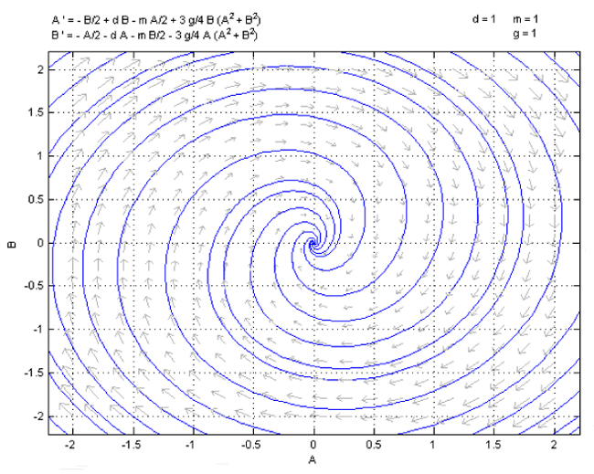 ) shows the case when α > 1/2. The diagram begins at the point (0.8,0), representing the value
  . After moving up to the line y = x at (0.8,0.8), the process then moves to the right to (1.1,0.8), where 1.1 represents the next value, . After several iterations, the values of approach the point (1.2,1.2), where 1.2 is the size of the stable limit cycle in this region.
 |
Fig. (8) Cobweb diagram for α = 0.6 and γ = 1. |
Fig. (9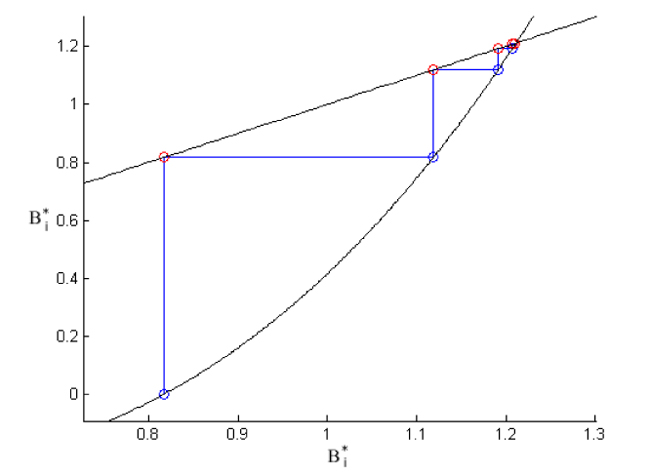 ) shows the case when α < -1/2. The diagram begins at the point (0.8,0), as before. This time, after moving up to the point (0.8,0.8), the process then moves to the left to (-1.2,0.8), where -1.2 represents the next value, . After several iterations, the values of alternate between two values, 1.3 and -1.3, reflecting the out-of-phase nature of the stable limit cycle in this region.
 |
Fig. (9) Cobweb diagram for α = -0.6 and γ = 1. |
For -1/2 < α < 1/2, there are three possible limit cycles. Since the output of eq. (23) is multi-valued in this region, there are many different cobweb diagrams for a given starting point , with the realized outcome determined by the initial condition in the original system (1, 2). The code used to generate the diagrams picks one of the three limit cycles at random, as this best represents the unpredictability of knowing the precise initial condition.
Fig. (10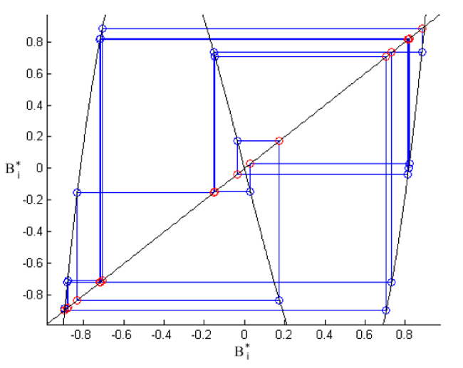 ) shows the chaotic nature of this iteration map in the region -1/2 < α < 1/2. Since the behavior here is randomized, there is no clear pattern to be discerned here. However, we note that the attractor seems to be a fractal of some kind since there are gaps that are never reached.
 |
Fig. (10) Cobweb diagram for α = 0.1 and γ = 1. |
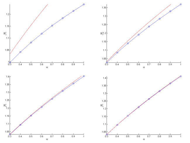 |
Fig. (11) Plots of vs α for α ≥ 0.3 and γ = 1. The top left graph shows n = 2, the top right graph shows n = 3, the bottom left graph shows n = 4, and the bottom right graph shows n = 5.
|
4.3. Convergence to the Limit
The most important question in this model is determining how long a train of bunches can be before the tail becomes unstable. We have shown that there is a theoretical upper bound to the limit cycle amplitude, but it remains to be seen how quickly the numerical sequence given by Eq. (23) approaches this limit.
Fig. (11 ) shows a sequence of graphs of vs α for 2 ≤ n ≤ 5 and α ≥ 0.3, which demonstrates the speed at which this sequence approaches the limit. However, we note that the sequence does not seem to converge pointwise at the same rate, and for larger α values, it takes longer to converge to the limit.
Fig. (12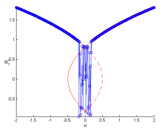 ) shows the graph of
  vs α for a larger range of α values, including the multi-valued region. While the multi-valued region does not show convergence to either of the limit curves, the values do stay bounded between the maximum values of the two limit curves. Thus, even in this region we, can place an upper bound on how large the can grow.
 |
Fig. (12) Plots of vs α for -2≤α≤2 and γ = 1.
|
Fig. (13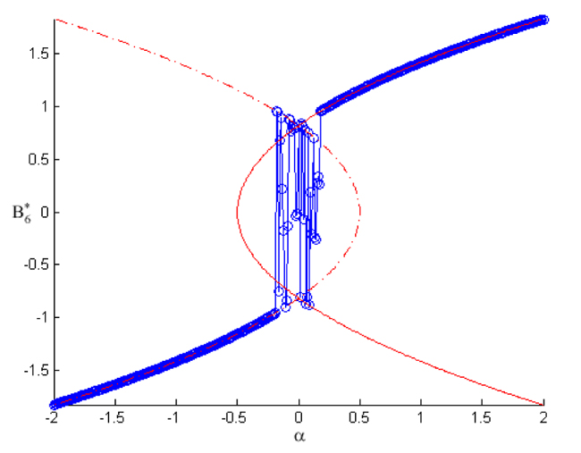 ) shows the graph of
  vs α. For α > 0.5, this figure is almost identical to Fig. (12), but for α < -0.5 the sign of the curve is now negative instead of positive. This reflects how the limit cycle in this region is out-of-phase, as is out of phase with . Since the magnitude of the limit curve is the same for both positive and negative branches, the sign of is of little concern.
 |
Fig. (13) Plots of vs α for -2≤α≤2 and γ = 1.
|
CONCLUSION
Our model predicts an upper bound for the amplitudes of bunches in a train. While the dynamics of the system varies depending on the value of α, the upper bound holds for all values of α.
In theory, this means that all trajectories are bounded, but in practice, there is a physical bound on how large amplitudes can grow before they become unstable. For example, if the theoretical bound on the motion is 100 centimeters, but the radius of the cross-section of the accelerator is only 2 centimeters, then instability occurs once grows larger than 2 centimeters. On the other hand, if the theoretical bound on the motion is 1 centimeter, then instability will never occur, as will never grow larger than 2 centimeters.
If it is known that the physical upper bound is smaller than the theoretical upper bound, then it is a simple matter to numerically calculate from eq. (23) and determine at what point exceeds the physical bound. Even in the multi-valued region, taking the worst-case scenario when the amplitude grows, the largest at each step will determine the critical n at which instability occurs. Thus, it is possible to know how many bunches to include in a train before instability occurs.
If this model proves accurate, then α can be used to determine the maximum number of bunches in a train. As α contains information for both the per-bunch charge and the per-bunch spacing, adjusting either of these specifications can adjust the value of α, and thus affect the size of the train.
CONSENT FOR PUBLICATION
Not applicable.
CONFLICT OF INTEREST
The authors declare no conflict of interest, financial or otherwise.
ACKNOWLEDGEMENTS
The authors would like to thank their colleagues J. Sethna, D. Rubin and D. Sagan for introducing us to the dynamics of the synchrotron and for their continued support in this research.
This work was partially supported by NSF Grant PHY-1549132.
REFERENCES
| [1] | J. Cuevas, L.Q. English, P.G. Kevrekidis, and M. Anderson, "Discrete breathers in a forced-damped array of coupled pendula: Modeling, computation, and experiment", Phys. Rev. Lett., vol. 102, no. 22, p. 224101. [http://dx.doi.org/10.1103/PhysRevLett.102.224101] [PMID: 19658866] |
| [2] | M. Syafwan, H. Susanto, and S.M. Cox, "Discrete solitons in electromechanical resonators", Phys. Rev. E Stat. Nonlin. Soft Matter Phys., vol. 81, no. 2 Pt 2, p. 026207. [http://dx.doi.org/10.1103/PhysRevE.81.026207] [PMID: 20365638] |
| [3] | C.S. Hsu, "On a restricted class of coupled Hill’s equations and some applications", J. Appl. Mech., vol. 28, no. 4, pp. 551-556. [http://dx.doi.org/10.1115/1.3641781] |
| [4] | A. Bernstein, and R.H. Rand, A. Bernstein, and R.H. Rand, "Coupled Parametrically Driven Modes in Synchrotron Dynamics", In: Proceedings of the 33rd IMAC, A
Conference and Exposition on Structural Dynamics, G. Kerschen, Ed., Springer: Newyork, 2016
[http://dx.doi.org/10.1007/978-3-319-15221-9_8] |
| [5] | I. Kovacic, R.H. Rand, and S.M. Sah, "Mathieu’s equation and its generalizations: Overview of stability charts and their features", Appl. Mech. Rev., vol. 70, no. 2, p. 020802. [http://dx.doi.org/10.1115/1.4039144] |
| [6] | G.M. Wang, T. Shaftan, V. Smaluk, Y. Li, and R. Rand, "Lossless crossing of a resonance stopband during tune modulation by synchrotron oscillations", New J. Phys., vol. 19, no. 9, p. 093010. [http://dx.doi.org/10.1088/1367-2630/aa8742] |
| [7] | "Cornell Electron Storage Ring", CLASSE: CESR. Cornell laboratory for accelerator-based sciences and education, . Available from: http://www.lepp.cornell.edu/Research/CESR/WebHome.html |
| [8] | J. Kevorkian, and J.D. Cole, Perturbation methods in applied mathematics.Applied Mathematical Sciences., vol. 34, Springer: Waltham, MA, . |
| [9] | R.H. Rand, Lecture Notes in Nonlinear Vibrations., Published on-line by The Internet-First University Press, . Available from: http://ecommons.library.cornell.edu/handle/1813/28989 |
| [10] | MATLAB v.7.5 by Mathworks; applet pplane7.m by Polking, J. C , Rice University, Department of Mathematics, Available from: http://math.rice.edu/∼dfield/dfpp.html |