- Home
- About Journals
-
Information for Authors/ReviewersEditorial Policies
Publication Fee
Publication Cycle - Process Flowchart
Online Manuscript Submission and Tracking System
Publishing Ethics and Rectitude
Authorship
Author Benefits
Reviewer Guidelines
Guest Editor Guidelines
Peer Review Workflow
Quick Track Option
Copyediting Services
Bentham Open Membership
Bentham Open Advisory Board
Archiving Policies
Fabricating and Stating False Information
Post Publication Discussions and Corrections
Editorial Management
Advertise With Us
Funding Agencies
Rate List
Kudos
General FAQs
Special Fee Waivers and Discounts
- Contact
- Help
- About Us
- Search


The Open Petroleum Engineering Journal
(Discontinued)
ISSN: 1874-8341 ― Volume 12, 2019
A New Method to Estimate Total Organic Carbon (TOC) Content, an Example from Goldwyer Shale Formation, the Canning Basin
Munther Alshakhs*, Reza Rezaee
Abstract
Background:
There is an increasing interest in the Goldwyer Formation of the Canning Basin as a potentially prospective shale play. This Ordovician shaly formation is one of the most prominent source rocks in the Canning Basin. One key property to evaluate the prospectivity of any shale oil or gas is its total organic carbon (TOC) richness.
Objectives:
This study investigates different TOC estimation techniques and validates the reliability of each, aiming to provide a best estimating approach for local and global applications.
Method:
The limited well distribution in the large area of the Canning Basin makes a basin-wide study not warranted at this stage. A focused look into the Barbwire Terrace was carried out instead. General TOC estimation methods, such as Schmoker and ∆logR were employed for TOC calculation. TOC relationships of single and multivariate regressions were also derived from wireline data and TOC rock sample measurements.
Results:
Both Schmoker and ∆logR methods tend to overestimate TOC when compared to the available Rock-Eval pyrolysis TOC measurements. The regression approach have shown to provide the best TOC estiamtes for wells in the Barbwire Terrace, where the best multiple regression approach for the terrace and global application was found to be the one derived from gamma-ray (GR), bulk density (RHOB), and sonic log transit time (DT).
Conclusion:
The generalized nature of the Schmoker method, as it provides a global relationship between density and TOC is probably the main reason why this approach does not provide a good fit in the case of the Goldwyer Formation. Furthermore, the uncertainty associated with the ∆logR method factors, such as the level of maturity (LOM), and resistivity and sonic baselines greatly influence the TOC estimation in this method, and hence, sometimes do not merit a reliable TOC estimation. The multiple regression approach have shown to be most accurate once lithology and compaction information (GR, RHOB, and DT) were incorporated in the regression process. TOC was reliably estimated for wells inside and outside the Barbwire Terrace, and also for wells of a global lacustrine shale. Such derivation have provided a more accurate technical assessment of the shale play and its prospectivity as a potential unconventional hydrocarbon resource.
Article Information

Identifiers and Pagination:
Year: 2017Volume: 10
First Page: 118
Last Page: 133
Publisher Id: TOPEJ-10-118
DOI: 10.2174/1874834101710010118
Article History:
Received Date: 11/01/2017Revision Received Date: 09/03/2017
Acceptance Date: 18/04/2017
Electronic publication date: 19/05/2017
Collection year: 2017
open-access license: This is an open access article distributed under the terms of the Creative Commons Attribution 4.0 International Public License (CC-BY 4.0), a copy of which is available at: https://creativecommons.org/licenses/by/4.0/legalcode. This license permits unrestricted use, distribution, and reproduction in any medium, provided the original author and source are credited.
* Address correspondence to this author at the 26 Dick Perry Avenue, Petroleum Engineering Department, Curtin University, Kensington WA 6152, Australia; Tel: +61 (0)414904145; E-mails: munther.alshakhs@postgrad.curtin.edu.au, munther@outlook.com
| Open Peer Review Details | |||
|---|---|---|---|
| Manuscript submitted on 11-01-2017 |
Original Manuscript | A New Method to Estimate Total Organic Carbon (TOC) Content, an Example from Goldwyer Shale Formation, the Canning Basin | |
BACKGROUND
The Canning Basin is the largest sedimentary basin in Western Australia underlying an area of more than 595 000 km2. A third of the basin is under water, with water depths reaching up to 1000 m. It is bounded by Precambrian Kimberley Block, Amadeus Basin, and the Pilbara and Musgrave Blocks from the north, east, and south, respectively. A shallow basement separates the Canning and Officer Basins in the southeast, (Fig. 1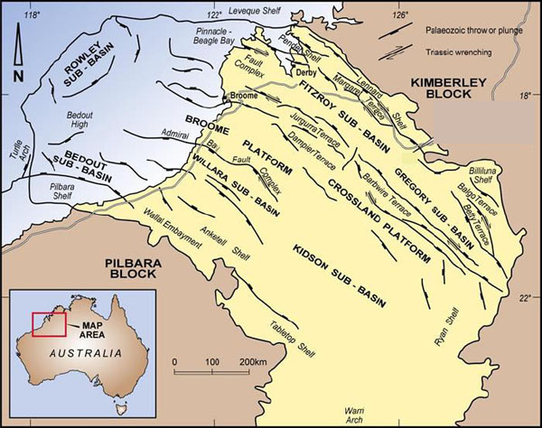 ) [1S. Cadman, L. Pain, V. Vuckovic, and S. Le Poidevin, "Canning Basin, W.A", Australian Petroleum Accumulation, Department of Primary Industries and Energy Bureau of Resource Sciences, Petroleum Resource Branch, no. 9, 1993.].
 |
Fig. (1) Tectonics and boundaries of the Canning Basin [1S. Cadman, L. Pain, V. Vuckovic, and S. Le Poidevin, "Canning Basin, W.A", Australian Petroleum Accumulation, Department of Primary Industries and Energy Bureau of Resource Sciences, Petroleum Resource Branch, no. 9, 1993.]. |
The stratigraphic column of the basin has a variable thickness that can reach up to 18 km of Ordovician to Quaternary sediments in some areas (Gregory Sub-basin) [1S. Cadman, L. Pain, V. Vuckovic, and S. Le Poidevin, "Canning Basin, W.A", Australian Petroleum Accumulation, Department of Primary Industries and Energy Bureau of Resource Sciences, Petroleum Resource Branch, no. 9, 1993.]. The deposition has started in the early Ordovician following a subsidence associated with regional rifting. The deposition of the multiple Ordovician formations took place under different marine settings. Two major halite units form a regional seal over the Ordovician deposits. The middle Ordovician Goldwyer Formation is the most prominent source rock in the section. The formation contains two major black shale sections with generally good quality oil-prone source rock that were deposited during peak transgressions [2P. Haines, and K. Ghori, "Rich Oil-prone Ordovician Source Beds, Bongabinni Formation, onshore Canning Basin, Western Australia", In: Extended Abstract: American Association of Petroleum Geologists, 2006.Perth, WAAAPG International Conference and Exhibition].
Average depth of the Goldwyer Formation is about 1330 m and average thickness is 350 m. TOC content in the Goldwyer Formation can be very variable and ranges from 0 to more than 6%. Estimations by Triche and Bahar [3N. Triche, and M. Bahar, "Shale Gas Volumetrics of Unconventional Resource Plays in the Canning Basin, Western Australia". Society of Petroleum Engineers (SPE). SPE-167078-MS, Brisbane, Australia, 11–13 November 2013.] suggest the initial gas-in-place of the lower Goldwyer Formation is about 867 Tcf (24.5 Tm3). Maturity data also suggest that the same unit could have shale oil potential in some parts of the basin [4 "Western Australia's Petroleum and Geothermal Explorer's Guide", Government of Western Australia, Department of Mines and Petroleum, 2014.].
METHOD
Total organic carbon content is a key factor in determining the prospectivity of any shale play. It significantly influences hydrocarbon production [5J. Schmoker, "Use of Formation-Density Logs to Determine Organic-Carbon Content in Devonian Shales of the Western Appalachian Basin and an Additional Example Based on the Bakken Formation of the Williston Basin", Petroleum Geology of the Black Shale of Eastern North America, 1989.]. TOC is traditionally measured in a laboratory from core data, sidewall plugs, and cuttings. This is relatively a more accurate method in TOC measurements. However, it provides non-continuous measurements of the source rock section as it has limited samples and is usually associated with higher costs and longer measurement time. To overcome these limitations, different continuous log data can be utilized to estimate TOC.
Petrophysical properties of the TOC vary greatly than those of the hosting source rock matrix. The presence of TOC generally coupled with higher gamma-ray (higher uranium content), lower density, higher resistivity, and slower sonic [6M. Kamali, and A. Allah Mirshady, "Total organic carbon content determined from well logs using ΔLogR and neuro fuzzy techniques", J. Petrol. Sci. Eng., vol. 45, no. 3-4, pp. 141-148, 2004.
[http://dx.doi.org/10.1016/j.petrol.2004.08.005] , 7S. Sun, Y. Sun, C. Sun, Z. Liu, and N. Dong, "Methods of Calculating Total Organic Carbon from Well Logs and its Application on Rock's Properties Analysis", Integration GeoConvention 2013, Geoscience Engineering Partnership, .]. Consequently, different methods and approaches were introduced to estimate TOC from well log data.
Schmoker’s method is a widely used one, and it estimates TOC from formation bulk density logs. Generally, a shale mineral matrix density has an average of 2.7 g/cc whereas organic matter has a density ranging from 1.2 to 1.4 g/cc. Thus, the presence of organic carbon will highly influence the formation bulk density and hence TOC is calculated from density-log when other factors for density variation are taken into consideration [8T. Hester, and J. Schmoker, "Determination of Organic Content From Formation-Density Logs, Devonian-Mississippian Woodford Shale, Anadarko Basin, Oklahoma", United States Geological Survey USGS, no. 87-20, 1987.].
This method subdivides shales into four components; rock matrix, pyrite, interstitial pores, and organic matter. Therefore, the bulk density of the formation is a function of those components and can be expressed as follows, Eq.1 [9J. Schmoker, and T. Hester, "Organic Carbon in Bakken Formation, United States Portion of Williston Basin", AAPG Bulletin, vol. 67, 1983.].
 |
(1) |
Ø = Volume fractions
ρb = Bulk density
m, p, i, and o are the matrix, pyrite, interstitial pores (pore fluid), and organic matter, respectively.
Schmoker [10J. Schmoker, "Determination of Organic Content of Appalachian Devonian Shales from Formation-Density logs: GEOLOGIC NOTES", AAPG Bulletin, vol. 63, 1979.] derived a linear relationship between pyrite and organic matter, empirically.
 |
(2) |
By assuming that the porosity changes in a shale rock are minimal and with low values to begin with, the porosity terms in eq. 1 can be eliminated. Additionally, by substituting eq. 2 in eq. 1, Hester and Schmoker [8T. Hester, and J. Schmoker, "Determination of Organic Content From Formation-Density Logs, Devonian-Mississippian Woodford Shale, Anadarko Basin, Oklahoma", United States Geological Survey USGS, no. 87-20, 1987.] have simplified and rearranged the relationship.
 |
(3) |
ρo = Density of organic matter
Øo = Organic matter volume fraction
This can be expressed in terms of TOC.
 |
(4) |
R = Ratio of weight percent organic matter to weight percent TOC
Schmoker has derived TOC equations for specific shales in North America. Eq. 4 is tailored for the Marcellus shale of the Appalachian Basin [5J. Schmoker, "Use of Formation-Density Logs to Determine Organic-Carbon Content in Devonian Shales of the Western Appalachian Basin and an Additional Example Based on the Bakken Formation of the Williston Basin", Petroleum Geology of the Black Shale of Eastern North America, 1989.]. By combining his different derivations for various shale plays [8T. Hester, and J. Schmoker, "Determination of Organic Content From Formation-Density Logs, Devonian-Mississippian Woodford Shale, Anadarko Basin, Oklahoma", United States Geological Survey USGS, no. 87-20, 1987.-10J. Schmoker, "Determination of Organic Content of Appalachian Devonian Shales from Formation-Density logs: GEOLOGIC NOTES", AAPG Bulletin, vol. 63, 1979.], we can use a more simplified/generalized version of his method, Eq. 5.
 |
(5) |
In [11Q. Passey, S. Creaney, J. Kulla, F. Moretti, and J. Stroud, "A practical model for organic richness from porosity and resistivity logs", AAPG Bulletin, vol. 74, no. 12, 1990.], the method proposed by Passey et al. was an advanced technique to estimate TOC compared to the simple estimation from density or gamma-ray logs [12B. Cluff, and M. Miller, "Logs Evaluation of Gas Shales: a 35-year Perspective", Presentation, April 2010 DWLS Luncheon, 2010.]. The (∆logR) technique of Passey et al. includes estimating TOC from three methods; sonic/resistivity, neutron/resistivity, and density/resistivity logs [6M. Kamali, and A. Allah Mirshady, "Total organic carbon content determined from well logs using ΔLogR and neuro fuzzy techniques", J. Petrol. Sci. Eng., vol. 45, no. 3-4, pp. 141-148, 2004.
[http://dx.doi.org/10.1016/j.petrol.2004.08.005] ]. The approach evolves around the log separation that occurs between the resistivity and the other logs, due to the presence of organic matter [7S. Sun, Y. Sun, C. Sun, Z. Liu, and N. Dong, "Methods of Calculating Total Organic Carbon from Well Logs and its Application on Rock's Properties Analysis", Integration GeoConvention 2013, Geoscience Engineering Partnership, .].
Taking the sonic/resistivity log method as an example, a separation between the two curves will be observed along the intervals of ‘hot’ shales (presence of organic matter). The two logs are overlayed on the same track, with the resistivity log displayed in logarithmic and the sonic in linear scales (Fig. 2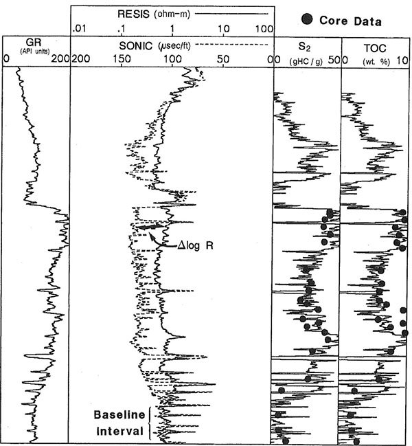 ). Slight modification to the scale length and interval might be required to emphasize the separation of the logs. The mathematical expression to quantify this separation is in Eq. 6 [11Q. Passey, S. Creaney, J. Kulla, F. Moretti, and J. Stroud, "A practical model for organic richness from porosity and resistivity logs", AAPG Bulletin, vol. 74, no. 12, 1990.].
 |
Fig. (2) Well logs illustrating how to estimate ∆logR from the separation between sonic and deep resistivity logs as outlined by the TOC estimation method of Passey et al. [11Q. Passey, S. Creaney, J. Kulla, F. Moretti, and J. Stroud, "A practical model for organic richness from porosity and resistivity logs", AAPG Bulletin, vol. 74, no. 12, 1990.]. |
 |
(6) |
∆logR is the separation between the two logs measured in logarithmic resistivity cycle.
R is the resistivity in Ω·m
∆t is the sonic measurement in µs/ft.
∆tbaseline is the sonic corresponding to Rbaseline in the lean shale interval (non-source rock).
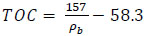
With the log separation quantified, the TOC can be calculated using Eq. 7.
 |
(7) |
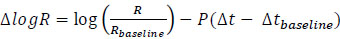
LOM is the level of maturity.
For any specific ∆logR, TOC decreases as LOM increases [12B. Cluff, and M. Miller, "Logs Evaluation of Gas Shales: a 35-year Perspective", Presentation, April 2010 DWLS Luncheon, 2010.]. LOM can be derived from maturity information (e.g. vitrinite reflectance Ro), see Fig. (3 ).
).
 |
Fig. (3) A 3rd degree polynomial expresses the relationship between Ro and LOM. |
There are some limitations associated with this Passey et al. approach. It might not be as reliable with high maturation levels, as resistivity logs do not continue increasing with maturity. They tend to fall back at some point of increasing maturity. Furthermore, TOC relationship was extrapolated after being derived and calibrated with low ∆logR and LOM 6-9. This again might pose some issues when dealing with values at the far end of the spectra [12B. Cluff, and M. Miller, "Logs Evaluation of Gas Shales: a 35-year Perspective", Presentation, April 2010 DWLS Luncheon, 2010.].
The two approaches of Schmoker and Passey et al. are considered the main techniques for TOC estimation. Such methods will be utilized in this study to calculate TOC and then will be validated with TOC measurements of rock samples. Moreover, those TOC measurements can also be cross-plotted with different petrophysical properties, like density and gamma-ray, to investigate the presence of any correlation.
Deriving TOC logs from available local log data can sometimes be a desirable approach. In many cases, this technique is more reliable than the previously discussed “one size fits all” approaches. Such method provides TOC logs derived from other local log data which are influenced by the TOC variation in the rock. Depending on correlation with TOC values from rock samples, techniques of single or multi-variate regressions can be utilized.
TOC Estimation
Schmoker and ∆logR Methods
There are 5 wells in the Barbwire Terrace with TOC measurements from Rock-Eval pyrolysis in the Goldwyer Formation, all of which have density logs. In a typical source rock, density logs are most sensitive to variations in TOC content. Hence, deriving TOC logs from density is a common practice.
Eq. 5 is a Schmoker linear regression between TOC and density, which was used to estimate TOC for Barbwire Terrace wells.
TOC was also estimated using Passey et al. (∆logR) method. This is a slightly more complicated approach, which requires deep resistivity and P-sonic logs. It also needs maturity information of Ro or Tmax data. Four wells in the Barbwire Terrace have the necessary data for TOC to be estimated from this method.
Calculated values of both methods overestimate TOC when validated against TOC measurements from Rock-Eval. This misfit is clearly observed in Fig. (4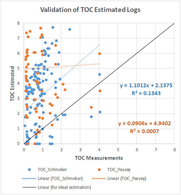 ), a cross plot between all estimated TOC values of both methods against TOC measurements from Rock-Eval. Fig. (5
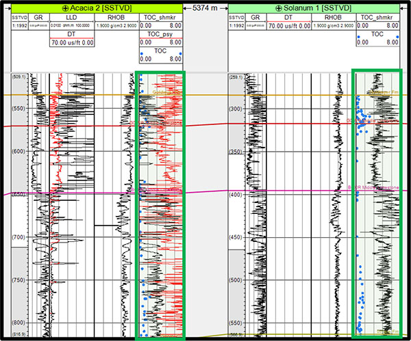 ) shows a cross section of two wells emphasizing the misfit caused when using the pre-defined TOC estimation methods.

It is noteworthy that applying ∆logR method has been suitable in other parts of the Canning Basin. This method has yielded acceptable TOC values in some areas of the Goldwyer Formation. However, such results mainly require manipulation of different ∆logR parameters that does not necessarily have any scientific basis. For example, available maturity data are not analysed and interpolated. They are often disregarded and simple manipulation of LOM is carried out instead. This simply entails changing the value of LOM for the whole section until the resultant log agrees the most with the TOC measurements. Such manipulations are not necessarily incorrect approaches, but they are not usually backed by sufficient scientific reasoning. For the purpose of this study, it was decided to prioritize exploring other TOC estimation options over the parameters manipulation of the pre-defined methods to deliver an adequate TOC solution of the Goldwyer Formation in the Barbwire Terrace, and possibly globally applicable.
Single and Multivariate Regression
With the pre-defined TOC methods not providing good estimates for the wells in the Barbwire Terrace, using local well data to derive TOC relationships has become more warranted. Multiple approaches were used, starting from a simple linear regression between Rock-Eval TOC measurements and density (RHOB). This can also be considered as adjusting Schmoker method parameters by utilizing data from the Goldwyer Formation in the Barbwire Terrace. Looking into the Rock-Eval TOC data, measurements were mainly taken from cuttings samples. As a result, depth of those samples cannot be exactly identified. It is very likely that those TOC points are not plotted against their correct corresponding densities. Depth values were edited based on the TOC values and density responses within a range of 10 ft (3 m), the standard range of error for cuttings depths (Fig. 6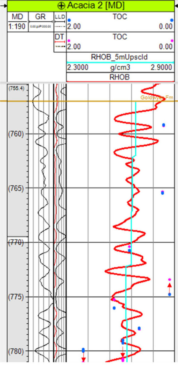 ). This depth matching exercise has substantially improved the correlation of TOC and density (Fig. 7
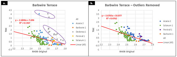 ).
).
 |
Fig. (5) Overestimating TOC-Schmoker (black) and TOC-Passey (red) when compared to TOC sample measurements (blue data points) in the tracks to the right for wells Acacia 2 and Solanum 1. |
 |
Fig. (6) Example of modifying the depths of the TOC measurements based on their values and density response. |
TOC data points of Dodonea 1 were treated as outliers and removed from the TOC-Density relationship of the Barbwire Terrace. Goldwyer thickness in this well is about 250 m, whereas all its 16 TOC data points were taken from a range of less than 15 m. TOC values are highly variable (from 0.6% to 4%) with small density variations. The quality of those measurements are questionable. One explanation of those anomalous data points is that they all lie in compositionally different facies zone, the generally kerogen-poor middle limestone zone of the Goldwyer section.
 |
Fig. (7) (a) TOC vs. RHOB for all wells in the Barbwire Terrace, after depth matching TOC measurements with density. (b) TOC vs. RHOB after depth matching and removing outliers. |
Consequently, TOC was derived from RHOB using the relationship between the two variables in Fig. (7b).
 |
(8) |
Once this single regression between TOC and RHOB was established (Eq. 8), multivariate regressions were also introduced to analyse any further improvement in TOC estimation. This included deriving TOC from gamma-ray and density, (Eq. 9).
 |
(9) |
TOC was also derived from gamma-ray, density, and neutron porosity. Eq. 10 shows this derivation.
 |
(10) |
Furthermore, other properties and different combinations were used to estimate TOC. Table 1 shows an extensive list of derived TOC equations, where the R2 associated with the cross-plot of calculated TOC versus measured TOC represents the estimated confidence of each approach.
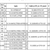
To further improve TOC estimation, the Goldwyer section was divided into 3 zones; upper, middle, and lower. The zoning was interpreted using log responses of common properties, such as gamma-ray, sonic, and density. Each zone had its own TOC estimation. The three zone and the one zone approaches were then calculated for those different combinations of multivariate regressions. All TOC estimations that involved neutron porosity (NPHI) are shown in Fig. (8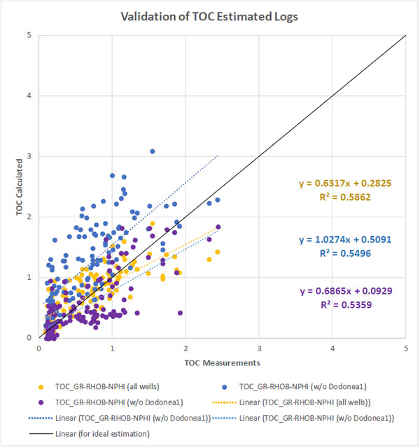 ). Whereas the validation of estimated TOC from other properties is illustrated in Fig. (9
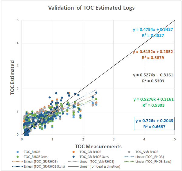 ). The best approach was identified to be the TOC estimated from density (RHOB) and gamma-ray (GR) for 3 zones in the Goldwyer, which when cross plotted against TOC values gives the highest R2, line slope closest to one, and has the lowest y-intercept value, closest to zero (Fig. 9). The one-zone approach of derived TOC log from the same properties, GR and RHOB, is the second best estimate.
 |
Fig. (8) TOC calculated from different regressions cross-plotted against measured TOC from Rock-Eval data. TOC values were estimated using gamma-ray, density, and neutron porosity. |
The three-zone approach derived three equations for TOC estimation from density and gamma-ray, one equation for each Goldwyer zone. These equations can be applied to all Barbwire Terrace wells to estimate TOC content of the Goldwyer Formation (Fig. 10 ).
).


DISCUSSION
As aforementioned, the GR-RHOB derived equations provide the best approach for TOC estimation in the Barbwire Terrace. However, when looking beyond the Goldwyer Formation and assessing the reliability of using this relationship to different shale types outside the Canning Basin, we might be missing something. Gamma-ray and density are properties that mostly representative of lithology. As lithology is a significant factor in shale evaluation, compaction can be just as significant. Practically, we could have two shale units with analogous lithology, and hence, similar RHOB and GR values but with different TOC values as they have different compaction/burial history.
For any TOC relationship, factors of both lithology and compaction should be represented for it to be more reliable globally, for different shales. We have generated such a relationship using compressional sonic as the compaction property, Eq. 11.
 |
(11) |
The resulted TOC log showed excellent correlation when cross-plotted against TOC measurements and overlayed in a well section along with other TOC log and measurement points, Figs. (11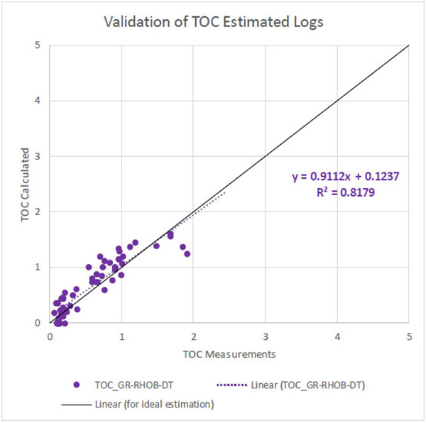 ) and (12
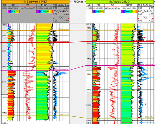 ), respectively. Estimated R2 of this equation is 0.82, suggesting that there is 82% confidence in this method for the estimation of TOC in the Barbwire Terrace. In other words, estimated error is 18%. Nevertheless, one well had to be dropped from the derivation as it had no sonic log transit time data across the Goldwyer Formation. Consequently, the apparent higher correlation can partially be regarded to the fewer data used. However, this is not the only reason for this correlation enhancement. We believe that the introduction of the compaction term to the equation is the main reason for the observed uplift, as we have now implemented both lithology and compaction information in the TOC estimation approach. Furthermore, the equation of derived TOC from GR, RHOB, and DT (Eq. 11) was applied to wells outside the Barbwire Terrace for further validation. Those wells are Crystal Creek 1 and Hilltop 1 of Mowla Terrace and Broom Platform, respectively. Derived TOC logs show good correlation with TOC data points (Fig. 13
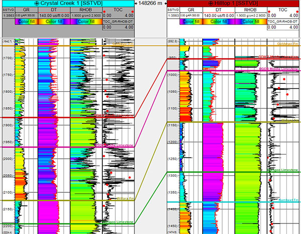 ).
).


The improvement in the TOC estimation after adding the compaction term is clearly evident. Such enhancements in the TOC estimation should also be observed when this relationship is applied for shale plays globally. Nonetheless, using a normalized gamma-ray can be more appropriate when applying the equation with the same constants to another shale formation. Consequently, eq. 11 can be updated to incorporate Vsh instead of GR (Eq. 12).
 |
(12) |
Vsh = Volume of shale (normalized gamma-ray)
Alternatively, in shale plays where sufficient data is available, deriving the source rock’s own constants can be even more reliable. The objective is to use key data of gamma-ray, density, and sonic transit time for TOC estimations where constants can change whenever appropriate (Eq. 13).
 |
(13) |
For a specific shale formation, either GR or Vsh (Eq.14) can be used for TOC estimation. Both equations (eq. 14 and eq. 13) can be used interchangeably as they would yield almost identical results.
 |
(14) |
EXAMPLE OF A GLOBAL SHALE APPLICATION
To further validate the findings of this study, TOC is estimated for a lacustrine shale in a different part of the world. This shale is very different from the Goldwyer Formation. The lacustrine source rock had been deposited in fluvial lacustrine settings during the Upper Triassic. Additionally, very high TOC values are measured from core samples, with TOC values averaging around 4.8%.
Given that sufficient number of TOC samples are available, TOC was estimated using eq.13. Parameters a, b, c, and d were all derived from the lacustrine data. For comparison, TOC was also estimated using different approaches, as multiple equations were derived from RHOB, GR, DT, and NPHI. Table 2 shows a list of these equations and their estimated parameters.
Estimated TOC values were then cross-plotted against TOC measurements to evaluate each estimation approach. TOC (Eq. 13) derived from gamma-ray, sonic transit time and density (GR, DT, & RHOB), once again, shows its superiority over other regressed properties, with estimated R2 of 0.79 (Fig. 14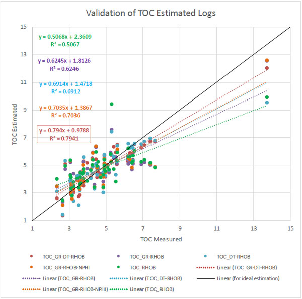 ). This further confirms that TOC derived from those three properties is prone to relatively provide most accurate regressed solution. A well cross section of the estimated log can be seen against core sample in Fig. (15
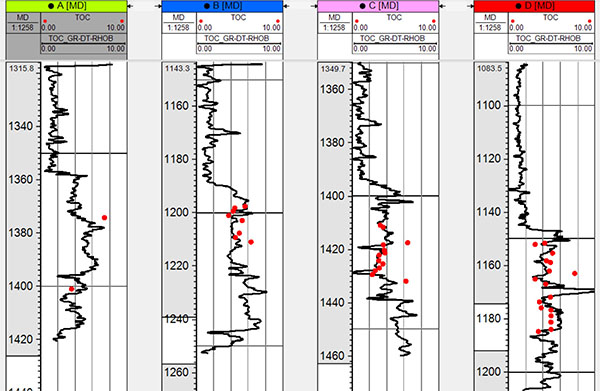 ).
).
CONCLUSION
In this study, pre-defined TOC estimation methods did not provide sufficient solutions for TOC. Their resultant TOC logs overestimated richness when compared to TOC measurements from rock samples. Linear and multivariate regressions provided a better fit for TOC estimation. With this approach, TOC can be derived from a wide range of logs. However, based on the common logs available in the Barbwire Terrace wells, deriving TOC from density and gamma-ray provided sufficiently well-validated TOC solution.
This relationship has improved when taking rock facies into account. A better solution was reached when the Goldwyer Formation was divided into three zones based on the interpretation of well log responses. Each zone had its own TOC – GR & RHOB relationship.
Data conditioning, however, was a very significant step to develop a relationship between TOC and any other property. Depth matching of TOC measurements to log responses has substantially improved the correlation. Nevertheless, such practices should only be carried out with care and rational justifications.
Using the introduced equations to estimate TOC for wells in the Canning Basin that are outside the Barbwire Terrace can be reasonable. However, given the complexity of the Canning Basin where the Goldwyer Formation can be highly variable in depth, thickness, kerogen type, maturity, and facies, it suggests that one TOC relationship might not be an appropriate solution for the Goldwyer across the whole basin. Instead, using established TOC estimation methods or introducing new relationships for deriving TOC from well logs can be more valid in areas with different Goldwyer characteristics.
As an attempt to deliver an equation that is more suitable for basin-wide and global applications, sonic log was introduced to the equation as a compaction term, complementing the other two lithology terms, gamma-ray and density (Eq. 11). The resultant TOC logs showed excellent correlation to the TOC measurements from Rock-Eval and suggest to work for wider shale types. This was further tested when TOC logs were properly estimated for two wells outside the Barbwire Terrace in the Canning Basin.


To further validate this concept, TOC values were estimated for a lacustrine shale. Equation 13 was utilized to estimate TOC, all parameters were derived from the TOC core measurements. This TOC log was then compared to TOC estimations derived from various regressions. The solution derived from eq. 13 still holds as the superior approach, further confirming that for TOC regression, using gamma-ray, density and sonic transit time provides an optimized TOC estimation.
CONFLICT OF INTEREST
The authors confirm that this article content has no conflict of interest.
ACKNOWLEDGEMENTS
We would like to acknowledge the help of Dr. Hongyan Yu in various aspects of the study. Our sincere thanks also goes to Schlumberger for their generous donation of Petrel licenses, and Saudi Aramco for sponsoring the author’s studies at Curtin University.
REFERENCES
| [1] | S. Cadman, L. Pain, V. Vuckovic, and S. Le Poidevin, "Canning Basin, W.A", Australian Petroleum Accumulation, Department of Primary Industries and Energy Bureau of Resource Sciences, Petroleum Resource Branch, no. 9, 1993. |
| [2] | P. Haines, and K. Ghori, "Rich Oil-prone Ordovician Source Beds, Bongabinni Formation, onshore Canning Basin, Western Australia", In: Extended Abstract: American Association of Petroleum Geologists, 2006.Perth, WAAAPG International Conference and Exhibition |
| [3] | N. Triche, and M. Bahar, "Shale Gas Volumetrics of Unconventional Resource Plays in the Canning Basin, Western Australia". Society of Petroleum Engineers (SPE). SPE-167078-MS, Brisbane, Australia, 11–13 November 2013. |
| [4] | "Western Australia's Petroleum and Geothermal Explorer's Guide", Government of Western Australia, Department of Mines and Petroleum, 2014. |
| [5] | J. Schmoker, "Use of Formation-Density Logs to Determine Organic-Carbon Content in Devonian Shales of the Western Appalachian Basin and an Additional Example Based on the Bakken Formation of the Williston Basin", Petroleum Geology of the Black Shale of Eastern North America, 1989. |
| [6] | M. Kamali, and A. Allah Mirshady, "Total organic carbon content determined from well logs using ΔLogR and neuro fuzzy techniques", J. Petrol. Sci. Eng., vol. 45, no. 3-4, pp. 141-148, 2004. [http://dx.doi.org/10.1016/j.petrol.2004.08.005] |
| [7] | S. Sun, Y. Sun, C. Sun, Z. Liu, and N. Dong, "Methods of Calculating Total Organic Carbon from Well Logs and its Application on Rock's Properties Analysis", Integration GeoConvention 2013, Geoscience Engineering Partnership, . |
| [8] | T. Hester, and J. Schmoker, "Determination of Organic Content From Formation-Density Logs, Devonian-Mississippian Woodford Shale, Anadarko Basin, Oklahoma", United States Geological Survey USGS, no. 87-20, 1987. |
| [9] | J. Schmoker, and T. Hester, "Organic Carbon in Bakken Formation, United States Portion of Williston Basin", AAPG Bulletin, vol. 67, 1983. |
| [10] | J. Schmoker, "Determination of Organic Content of Appalachian Devonian Shales from Formation-Density logs: GEOLOGIC NOTES", AAPG Bulletin, vol. 63, 1979. |
| [11] | Q. Passey, S. Creaney, J. Kulla, F. Moretti, and J. Stroud, "A practical model for organic richness from porosity and resistivity logs", AAPG Bulletin, vol. 74, no. 12, 1990. |
| [12] | B. Cluff, and M. Miller, "Logs Evaluation of Gas Shales: a 35-year Perspective", Presentation, April 2010 DWLS Luncheon, 2010. |