- Home
- About Journals
-
Information for Authors/ReviewersEditorial Policies
Publication Fee
Publication Cycle - Process Flowchart
Online Manuscript Submission and Tracking System
Publishing Ethics and Rectitude
Authorship
Author Benefits
Reviewer Guidelines
Guest Editor Guidelines
Peer Review Workflow
Quick Track Option
Copyediting Services
Bentham Open Membership
Bentham Open Advisory Board
Archiving Policies
Fabricating and Stating False Information
Post Publication Discussions and Corrections
Editorial Management
Advertise With Us
Funding Agencies
Rate List
Kudos
General FAQs
Special Fee Waivers and Discounts
- Contact
- Help
- About Us
- Search


The Open Petroleum Engineering Journal
(Discontinued)
ISSN: 1874-8341 ― Volume 12, 2019
Horizontal Bedding Shale Geostress Calculation Method
Zhang Ligang*, Qu Sining, Yan Tie, Guan Bing
Abstract
Background:
Since the fragile anisotropy of shale, it is difficult to carry out laboratory experiments of geostress by shale cores. The existing geostress calculation model that is based on the homogeneous hypothesis also cannot meet the accuracy requirement. Therefore, it is necessary to establish the new geostress calculation model and test methods which are suitable for shale and provide the effective guidance for drilling and fracturing.
Methods:
Firstly, the triaxial stress experiments were carried out. It showed that the mechanical parameters had strong difference between parallel and vertical bedding direction. The characteristics of transversely isotropic were shown obviously. Then, the geostress calculation model which considers the mechanical parameters of anisotropy in different direction was established by the constitutive relation of transversely isotropic materials. Finally, it was assumed that there is no relative displacement between formations in the process of deposition and the late tectonic movement; the prediction method for the shale geostress was established by the adjacent homogeneous formation. The sensitivity factors and influence laws were analyzed for the horizontal bedding shale geostress.
Results:
The results showed that the shale geostress was controlled by the elastic parameters of its own and the adjacent beds’.
Conclusion:
The research can provide the theoretical basis and easy way for calculating the shale geosterss.
Article Information

Identifiers and Pagination:
Year: 2017Volume: 10
First Page: 143
Last Page: 151
Publisher Id: TOPEJ-10-143
DOI: 10.2174/1874834101710010143
Article History:
Received Date: 15/08/2016Revision Received Date: 11/01/2017
Acceptance Date: 14/02/2017
Electronic publication date: 31/05/2017
Collection year: 2017
open-access license: This is an open access article distributed under the terms of the Creative Commons Attribution 4.0 International Public License (CC-BY 4.0), a copy of which is available at: https://creativecommons.org/licenses/by/4.0/legalcode. This license permits unrestricted use, distribution, and reproduction in any medium, provided the original author and source are credited.
* Address correspondence to this author the School of Petroleum Engineering, Northeast Petroleum University, Daqing 163318, Hei Longjiang Province, P.R. China, Tel: +96-04576502953; E-mail: zhangligang@163.com
| Open Peer Review Details | |||
|---|---|---|---|
| Manuscript submitted on 15-08-2016 |
Original Manuscript | Horizontal Bedding Shale Geostress Calculation Method | |
1. INTRODUCTION
The geosterss calculation model is able to reflect geosterss' physical nature and actual regularity. So far, a lot of scholars have established many geosterss calculation models, which include, Kinnick model [1Z.M. Li, and J.Z. Zhang, In-stiu Stress and Petroleum Exploration and Development, Petroleum Industry Press: China, 1997.], Mattews and Kelly model [2W.R. Matthews, and J. Kelly, "How to predict formation pressure and fracture gradient", Oil Gas J., vol. 65, no. 8, pp. 92-106, 1967.], Terzaghi model and Anderson model [3R.A. Anderson, D.S. Ingram, and A.M. Zanier, "Determining fracture pressure gradient from well logs", JPT, pp. 1259-1268, 1973.], Newberry model and Huang Rongzun model [4R.Z. Huang, "A model for predicting formation fracture pressure", J. Uni. Petrol. China, vol. 4, pp. 335-347, 1984.]. Although these models have considered the composition characteristics of geosterss in different aspects, the rocks were mostly treated as a homogeneous isotropic linear elastic material [5J.W. Cho, H. Kim, S. Jeon, and K.B. Min, "Deformation and strength anisotropy of Asan gneiss, Boryeong shale, and Yeoncheon schist", Int. J. Rock Mech. Min., vol. 50, pp. 158-169, 2012.
[http://dx.doi.org/10.1016/j.ijrmms.2011.12.004] -7Y. Deng, R. Guo, Z. Tian, C. Xiao, H. Han, and W. Tan, "Productivity model for shale gas reservoir with comprehensive consideration of multi-mechanisms", TOPEJ, vol. 8, no. 1, pp. 235-247, 2015.
[http://dx.doi.org/10.2174/1874834101508010235] ]. Due to the anisotropic characteristics of shale [8C.D. Piane, D.N. Dewhurst, A.F. Siggins, and M.D. Raven, "Stress-induced anisotropy in saturated shale", Geophys. J. Int., vol. 184, no. 2, pp. 897-906, 2011.
[http://dx.doi.org/10.1111/j.1365-246X.2010.04885.x] -11S. Stackhouse, "First-principles calculation of the elastic moduli of sheet silicates and their application to shale anisotropy", Am. Mineral., vol. 96, no. 1, pp. 125-137, 2011.
[http://dx.doi.org/10.2138/am.2011.3558] ], there was lack of accuracy in the above mentioned models, and were no longer suitable for horizontal bedding shale [12C.M. Sayers, "Seismic anisotropy of shales", Geophys. Prospect., vol. 53, no. 5, pp. 667-676, 2005.
[http://dx.doi.org/10.1111/j.1365-2478.2005.00495.x] , 13R. Gautam, "Anisotropy in deformations and hydraulic properties of Colorado shale", PhD Thesis, University of Calgary, Canada, 2014.]. In addition, due to fragile shale core, the coring and the process of making specimen were difficult [14F. Yang, Z. Ning, C. Hu, B. Wang, K. Peng, and H. Liu, "Characterization of microscopic pore structures in shale resercoirs", Acta Petrol. Sin., vol. 34, no. 2, pp. 301-311, 2013., 15J. Guo, J. Yin, and Z. Zhao, "Feasibility of formation of complex fractures under cracks interference in shale reservoir fracturing", Chinese J. Rock Mech. Eng., vol. 33, no. 8, pp. 1589-1596, 2014.]. The laboratory experiment (Viscous remanent magnetization, DSA) [16F.D. Strickland, and N.K. Ran, "Predicting the in-situ stress for deep wells using differential strain curve analysis", In: SPE8954, 1980, pp. 251-255.
[http://dx.doi.org/10.2118/8954-MS] -20K. Zhao, D.Q. Yan, C.H. Zhong, X.Y. Zhi, X.J. Wang, and X.Q. Xiong, "Comprehensive analysis method and experimental vertification for in-situ stress measurement by acoustic emission tests", Chinese J. Geotech. Eng., vol. 34, no. 8, pp. 1403-1411, 2012.] and other experiment of geostress with core was more difficult. Therefore, it is necessary to carry on the research for the geosterss calculation model and retrieval method of horizontal beddings shale.
2. THE EXPERIMENT OF MECHANICAL PROPERTIES
The shale rock mass has good bedding structure, which leads to anisotropy of the mechanical properties of shale. The horizontal bedding shale of Liaohe Oilfield was selected as the research object. The bedding developmental state is shown in Fig. (1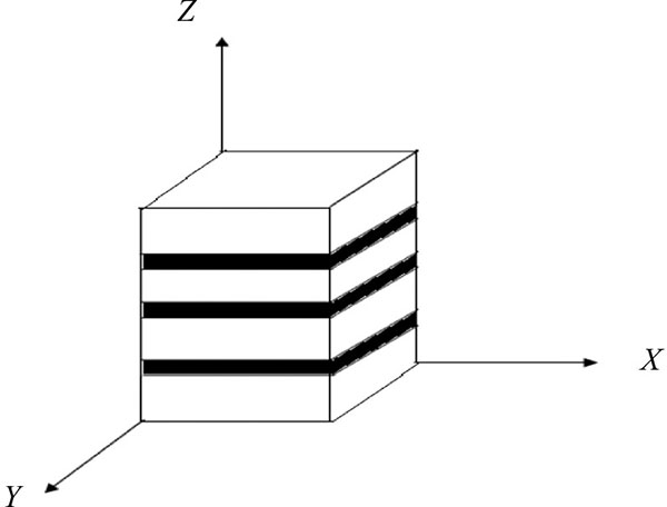 ). The dry samples of shale were cored along the X`Y`Z directions selectively. All cylindrical specimens with the height to diameter ratio of 2 (±0.03) were prepared by cutting and polishing. The triaxial stress experiments were carried out with the machine of RAW2000. The full stress-strain curves and fracture morphologies were obtained. The results of Z1-1 are shown in Fig. (2
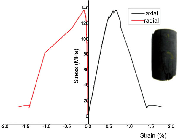 ).
).
 |
Fig. (1) The horizontal bedding shale diagram. |
 |
Fig. (2) Full stress-strain curve and fracture of Z1-1. |
According to the full stress-strain curves of each rock specimen, the elastic modulus, Poisson's ratio and compressive strength were calculated in X, Y, and Z directions. The results are shown in Table 1.
The results showed that the values of elastic parameters that are parallel to the bedding plane (along the X and Y direction) were close, and which had large differences from the vertical to bedding plane (Z direction). The vertical values were significantly higher than the parallel values. The rock presents the feature of transversely isotropic.
3. THE GEOSTRESS CALCULATION MODEL
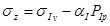
3.1. Vertical Geosterss Calculation Model
The geologists of Heim and Swiss assumed that the vertical geosterss is caused by overlying formation gravity [1Z.M. Li, and J.Z. Zhang, In-stiu Stress and Petroleum Exploration and Development, Petroleum Industry Press: China, 1997.]. The value changes with the formation density and depth. Therefore, the vertical geosterss can be calculated by density log information.
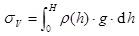 |
(1) |
The actual formation density varies with the depth, which is difficult to use a simple function to represent. According to the density logs, the average density of a hole section can be obtained. So it can be calculated by the method of subsection summation.
 |
(2) |
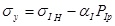
3.2. Horizontal Geosterss Calculation Model
The horizontal bedding shale can be seen as transversely isotropic material, and the constitutive equation can be expressed as:
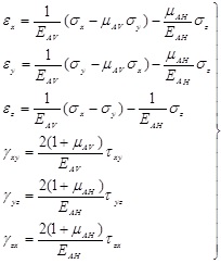 |
(3) |
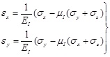
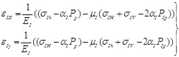
Generally, three directions X, Y, Z are the main stress directions and the vertical stress is the overburden pressure. According to the constitutive equation, the effective stresses of two horizontal directions can be derived as:
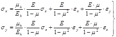 |
(4) |
Where
 ,
,
 and
and
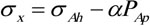
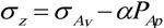 , the horizontal geosterss calculation model can be written as:
 |
(5) |
3.3. Geosterss Calculation Model by Adjacent Homogeneous Formations
Due to the fragile nature of the shale rock, the calculation model is established to invert the horizontal bedding shale geostress by using the adjacent homogeneous formation. It was assumed that there is no relative displacement between the formations and the strains are constant in two horizontal directions in all formations in the process of deposition and the late tectonic movement. The constitutive model of the homogeneous isotropic formations is obtained as:
 |
(6) |
Where
 ,
,
 and
and
 , the strain of the adjacent homogeneous formation can be gotten as:
 |
(7) |
Ordering the
 and
and
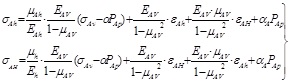
 and substituting the strain of the adjacent formations into the (5), the horizontal bedding shale geosterss can be calculated as:
 |
(8) |
4. THE DISCUSSION OF SENSITIVITY FACTORS AND INFLUENCE LAWS
The depth of the shale coring layer was 1600m. In the vertical direction to the bedding plane, the elastic modulus is 15097.8MPa and the Poisson's ratio is 0.32. In the direction of parallel to the bedding plane, the elastic modulus is 8790.9MPa and the Poisson's ratio is 0.36. In the adjacent homogeneous formations, the elastic modulus is 30927.3MPa and the Poisson's ratio is 0.22. The single factor was varied, the sensitivity factors and influence laws were determined simultaneously.
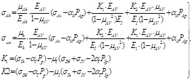
With the elastic modulus and Poisson's ratio of the vertical bedding direction increased, the in-stiu stress of two horizontal directions increased linearly as shown in Fig. (3a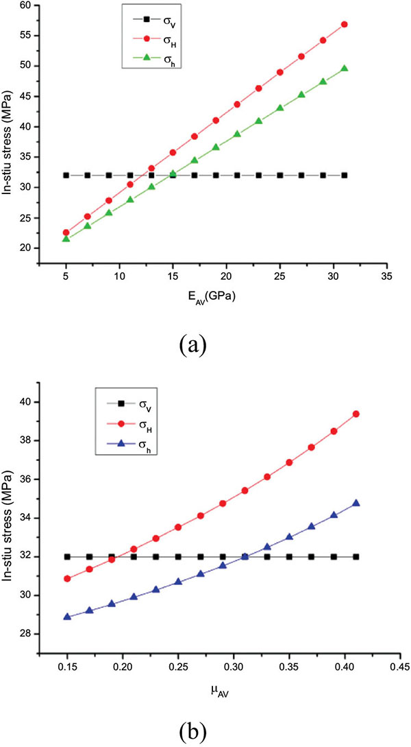 ). With the increased Poisson's ratio, the geostress of two horizontal direction increased exponentially. The growth rate was higher for the maximum horizontal geostress. The difference between two horizontal geosterss increases gradually as shown in Fig. (3b).
 |
Fig. (3) The sensitivities for the elastic parameters of the vertical bedding direction. |
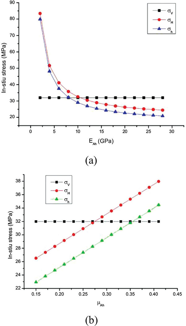 |
Fig. (4) The sensitivities for the elastic parameters of the parallel bedding direction. |
With the increased elastic modulus of parallel vertical bedding direction, the in-situ stress of two horizontal directions was decreasing exponentially and the decrease rate of the minimum horizontal geostress was bigger, as shown in Fig. (4a ). With the Poisson's ratio increased, the geostress of the two horizontal direction was increased linearly, the growth rate of two horizontal geostress is similar as shown in Fig. (4b).
With the increased elastic modulus of the adjacent homogeneous formations, the in-situ stress of two horizontal direction decreased exponentially. The decrease rate of maximum horizontal geostress was faster. The difference between the two horizontal geostress decreased gradually, and finally became equal, as shown in Fig. (5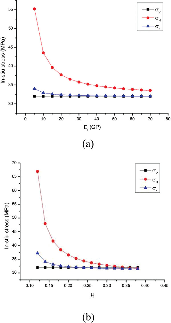 ). The main reason was that, the adjacent formation had stronger ability to resist deformation and bear more tectonic stress.
 |
Fig. (5) The sensitivities for the elastic parameters of the adjacent homogeneous formations. |
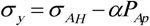
5. ENGINEERING APPLICATION
When using the new method to predict the shale geostress by the adjacent homogeneous formation, the following procedures should be obeyed.
- Combining with the indoor experiments or logging data, the shale elastic parameters of the vertical direction, parallel direction and the adjacent homogeneous formations should be calculated.
- The geosterss of the adjacent homogeneous formations should be evaluated by the small scale fracturing or the laboratory experiment.
- By appling the new calculation model, the geostress of the horizontal bedding shale can be obtained.
Based on the above procedures, the shale geostress of Liaohe Oilfield was calculated. Firstly, the sandstones adjacent with the shale were cored and the DSA experiment was carried out. The DSA experimental apparatus and rock specimens are shown in Fig. (6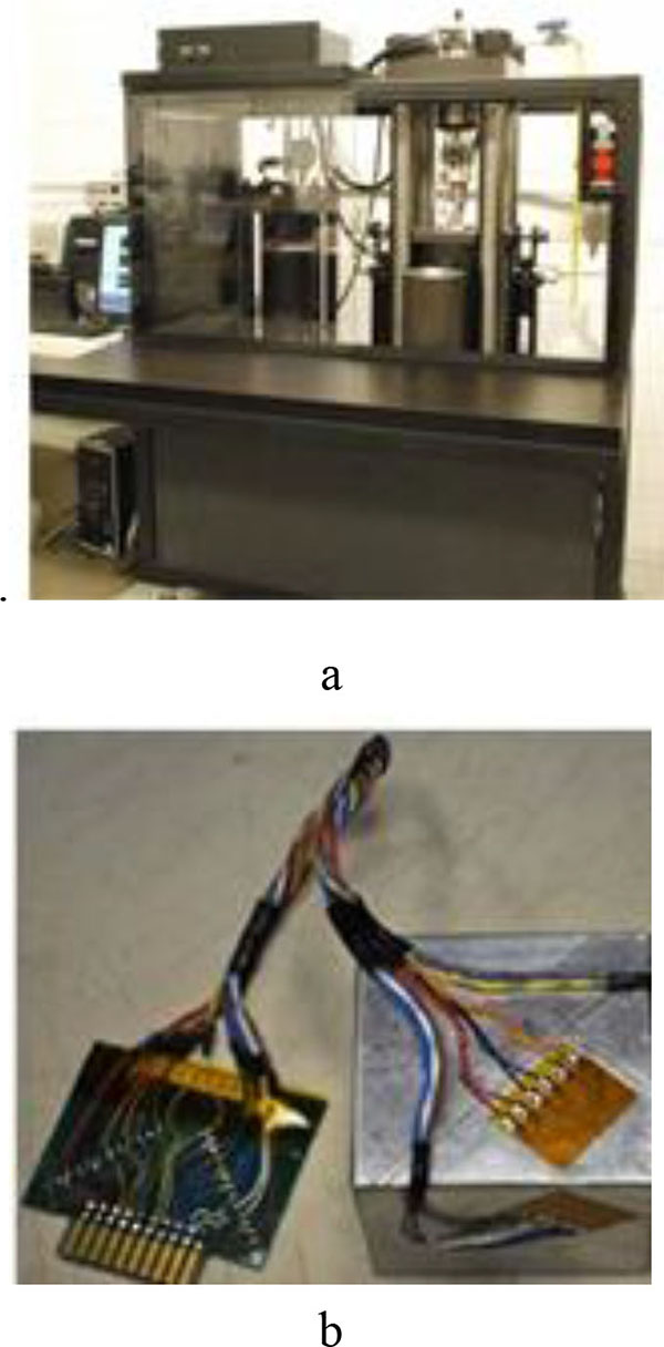 ).
).
 |
Fig. (6) The DSA test apparatus and specimen. |
The vertical stress was 30.5 MPa. The maximum horizontal geostress was 36.2 MPa and the minimum horizontal geostress was 24.8 MPa. According to the geostress of the measuring point, the geostress of the shale layer was calculated by combining with Terzaghi model, Newberry model, Huang Rongzun model and the new model established in this paper. The results are shown in Fig. (7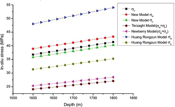 ).
).
 |
Fig. (7) The results calculated by different model. |
Without considering the influence of tectonic stress, the calculation result of geostress by Terzaghi and Newberry model was lower. In the Huang Rongzun model, only considering the effect of Poisson's ratio, it was concluded that the maximum horizontal geostress value was larger and the minimum horizontal geostress value was smaller without the effect of elastic modulus. The new model considered the influence of Poisson's ratio and elastic modulus simultaneously. Thus, the calculation results were in the range of the results of Huang Rongzun model.
CONCLUSION
- Considered the transversely isotropic characteristics, the new geostress calculation model and prediction method were established. The model and method were more convenient and precise for the horizontal bedding shale.
- The sensitivity factors and influence laws were analyzed. The major influences of the shale geostress were the elastic parameters of its own and those of the adjacent bed. The accurate evaluation of the mechanical parameters of shale and adjacent layers provides a basis for calculating the shale geostress.
NOMENCLATURE AND UNITS
| H | = Burial depth of formation m |
| P(h) | = The function about formation density changing with formation depth |
| g | = Acceleration of gravity g/cm3 |
| ΔDi | = Thickness of the i segment m |
| ρi | = Average bulk density of the i segment in density logs g/cm3 |
| σAV | = Overburden pressure in the shale formation MPa |
| σAH | = The maximum horizontal stress in the shale formation MPa |
| σAh | = The minimal horizontal stress in the shale formation MPa |
| σAIV | = Overburden pressure in the adjacent homogeneous formation MPa |
| σAIV | = The maximum horizontal stress in the adjacent homogeneous formation MPa |
| σAH | = The minimal horizontal stress in the adjacent homogeneous formation MPa |
| PAP | = Pore pressure in the shale formation MPa |
| PIP | = Pore pressure in the adjacent homogeneous formation MPa |
| EAV | = Elastic Modulus vertical to bedding direction MPa |
| µAV | = Poisson's ratio vertical to bedding direction |
| EAh | = Elastic Modulus parallel to bedding direction MPa |
| µAh | = Poisson's ratio parallel to bedding direction |
| E1 | = Elastic Modulusof the adjacent homogeneous formation MPa |
| µAh | = Poisson's ratioof the adjacent homogeneous formation |
| αA | = Biot coefficient of the shale formation |
| α1 | = Biot coefficient of the adjacent homogeneous formation |
| K1 ` K2 | = The middle transition coefficient. |
CONFLICT OF INTREST
The authors confirm that this article content has no conflict of interest.
ACKNOWLEDGEMENTS
The research was supported by NSFC (Natural Science Foundation of China, No. 51504067 and No.51490650) and Postdoctoral foundation of Heilongjiang Province (No.LBH-Z15031) in the context of Northeast Petroleum University.
REFERENCES
| [1] | Z.M. Li, and J.Z. Zhang, In-stiu Stress and Petroleum Exploration and Development, Petroleum Industry Press: China, 1997. |
| [2] | W.R. Matthews, and J. Kelly, "How to predict formation pressure and fracture gradient", Oil Gas J., vol. 65, no. 8, pp. 92-106, 1967. |
| [3] | R.A. Anderson, D.S. Ingram, and A.M. Zanier, "Determining fracture pressure gradient from well logs", JPT, pp. 1259-1268, 1973. |
| [4] | R.Z. Huang, "A model for predicting formation fracture pressure", J. Uni. Petrol. China, vol. 4, pp. 335-347, 1984. |
| [5] | J.W. Cho, H. Kim, S. Jeon, and K.B. Min, "Deformation and strength anisotropy of Asan gneiss, Boryeong shale, and Yeoncheon schist", Int. J. Rock Mech. Min., vol. 50, pp. 158-169, 2012. [http://dx.doi.org/10.1016/j.ijrmms.2011.12.004] |
| [6] | H. Sone, and M.D. Zoback, "Time-dependent deformation of shale gas reservoir rocks and its long-term effect on the in situ state of stress", Int. J. Rock Mech. Min., vol. 69, no. 3, pp. 120-132, 2014. |
| [7] | Y. Deng, R. Guo, Z. Tian, C. Xiao, H. Han, and W. Tan, "Productivity model for shale gas reservoir with comprehensive consideration of multi-mechanisms", TOPEJ, vol. 8, no. 1, pp. 235-247, 2015. [http://dx.doi.org/10.2174/1874834101508010235] |
| [8] | C.D. Piane, D.N. Dewhurst, A.F. Siggins, and M.D. Raven, "Stress-induced anisotropy in saturated shale", Geophys. J. Int., vol. 184, no. 2, pp. 897-906, 2011. [http://dx.doi.org/10.1111/j.1365-246X.2010.04885.x] |
| [9] | H. Kim, J.W. Cho, I. Song, and K.B. Min, "Anisotropy of elastic moduli, p-wave velocities, and thermal conductivities of asan gneiss, boryeong shale and Yeoncheon Schist in Korea", Eng. Geol., vol. 147-148, no. 5, pp. 68-77, 2012. [http://dx.doi.org/10.1016/j.enggeo.2012.07.015] |
| [10] | Z. Kai, J.G. Deng, T. Qiang, B.H. Yu, J.L. Yuan, and H.Y. Zhu, "Borehole stability in shale formation for extended reach wells", TOPEJ, vol. 5, pp. 130-137, 2014. [http://dx.doi.org/10.2174/1874834101205010130] |
| [11] | S. Stackhouse, "First-principles calculation of the elastic moduli of sheet silicates and their application to shale anisotropy", Am. Mineral., vol. 96, no. 1, pp. 125-137, 2011. [http://dx.doi.org/10.2138/am.2011.3558] |
| [12] | C.M. Sayers, "Seismic anisotropy of shales", Geophys. Prospect., vol. 53, no. 5, pp. 667-676, 2005. [http://dx.doi.org/10.1111/j.1365-2478.2005.00495.x] |
| [13] | R. Gautam, "Anisotropy in deformations and hydraulic properties of Colorado shale", PhD Thesis, University of Calgary, Canada, 2014. |
| [14] | F. Yang, Z. Ning, C. Hu, B. Wang, K. Peng, and H. Liu, "Characterization of microscopic pore structures in shale resercoirs", Acta Petrol. Sin., vol. 34, no. 2, pp. 301-311, 2013. |
| [15] | J. Guo, J. Yin, and Z. Zhao, "Feasibility of formation of complex fractures under cracks interference in shale reservoir fracturing", Chinese J. Rock Mech. Eng., vol. 33, no. 8, pp. 1589-1596, 2014. |
| [16] | F.D. Strickland, and N.K. Ran, "Predicting the in-situ stress for deep wells using differential strain curve analysis", In: SPE8954, 1980, pp. 251-255. [http://dx.doi.org/10.2118/8954-MS] |
| [17] | S. Lin, Z. Xudong, and J. Yan, "New method for measurement of in-situ stresses at great depth", Chinese J. Rock Mech. Eng., vol. 23, no. 14, pp. 2355-2358, 2004. |
| [18] | L.G. Zhang, H.B. Wang, X.D. Si, and S.B. Li, "The experimental study on the in-situ stress of Song Nan block", Appl. Mech. Mater., vol. 395-396, pp. 852-855, 2013. [http://dx.doi.org/10.4028/www.scientific.net/AMM.395-396.852] |
| [19] | B.K. Sinha, and T.J. Plona, "Wave propagation in rocks with elastic-plastic deformations", Geophysics, vol. 66, no. 3, pp. 772-785, 2001. [http://dx.doi.org/10.1190/1.1444967] |
| [20] | K. Zhao, D.Q. Yan, C.H. Zhong, X.Y. Zhi, X.J. Wang, and X.Q. Xiong, "Comprehensive analysis method and experimental vertification for in-situ stress measurement by acoustic emission tests", Chinese J. Geotech. Eng., vol. 34, no. 8, pp. 1403-1411, 2012. |