- Home
- About Journals
-
Information for Authors/ReviewersEditorial Policies
Publication Fee
Publication Cycle - Process Flowchart
Online Manuscript Submission and Tracking System
Publishing Ethics and Rectitude
Authorship
Author Benefits
Reviewer Guidelines
Guest Editor Guidelines
Peer Review Workflow
Quick Track Option
Copyediting Services
Bentham Open Membership
Bentham Open Advisory Board
Archiving Policies
Fabricating and Stating False Information
Post Publication Discussions and Corrections
Editorial Management
Advertise With Us
Funding Agencies
Rate List
Kudos
General FAQs
Special Fee Waivers and Discounts
- Contact
- Help
- About Us
- Search


The Open Petroleum Engineering Journal
(Discontinued)
ISSN: 1874-8341 ― Volume 12, 2019
Implementation of Region-Based Covariance Localization Ensemble Kalman Filter in History Matching Workflow
Fajril Ambia1, *, Tutuka Ariadji1, Zuher Syihab1, Agus Y. Gunawan2
Abstract
Background:
History matching is an indispensable phase in the workflow of reservoir analysis. Nevertheless, there is a considerable challenge in performing the procedure in a proper scientific manner due to the inherent nature of non-unique solutions from the many-unknown variables with limited known equations.
Objective:
In this study, we introduce the Ensemble Kalman Filter (EnKF) method complemented by the Region-Based Covariance Localization (RCL) scheme to address the aforementioned issue.
Method:
The algorithms work initially by modifying the covariance localization generated by Gaussian correlation model using region information such as facies or flow unit, in which the area within a region is spatially correlated. Subsequently, the correlation between distant areas in the region is eliminated, hence promoting better modification of the distribution of the parameters while maintaining the characteristics of the predefined geological model of the reservoir.
Result:
Result shows that RCL scheme is capable of enhancing the performance of EnKF procedure and produce parameter distributions that is close to the true model of the reservoir.
Conclusion:
Implementation of the proposed methodology ameliorates the accuracy and reliability of the history matching process, thus establishing better consideration in predicting reservoir performance.
Article Information

Identifiers and Pagination:
Year: 2017Volume: 10
First Page: 177
Last Page: 194
Publisher Id: TOPEJ-10-177
DOI: 10.2174/1874834101710010177
Article History:
Received Date: 18/02/2017Revision Received Date: 05/06/2017
Acceptance Date: 20/06/2017
Electronic publication date: 29/08/2017
Collection year: 2017
open-access license: This is an open access article distributed under the terms of the Creative Commons Attribution 4.0 International Public License (CC-BY 4.0), a copy of which is available at: https://creativecommons.org/licenses/by/4.0/legalcode. This license permits unrestricted use, distribution, and reproduction in any medium, provided the original author and source are credited.
* Address correspondence to this author at the Faculty of Mining and Petroleum Engineering, Institut Teknologi Bandung,Jawa Barat 40132, Indonesia; Tel: +628119401357; E-Mail: fajril@ambia.id
| Open Peer Review Details | |||
|---|---|---|---|
| Manuscript submitted on 18-02-2017 |
Original Manuscript | Implementation of Region-Based Covariance Localization Ensemble Kalman Filter in History Matching Workflow | |
1. INTRODUCTION
History matching is an essential phase in reservoir dynamic modeling workflow. The aim of history matching is to generate the most appropriate reservoir model that would provide prediction as close as possible to the acquired production data [1Z. Tavassoli, J.N. Carter, and P.R. King, "Errors in history matching", SPE J., pp. 352-361, 2004.
[http://dx.doi.org/10.2118/86883-PA] ]. Static parameters in a reservoir model that usually need to be tuned in history matching process are skin factor, permeability thickness, vertical to horizontal permeability ratio and aquifer constant. Usually, these parameters were assigned as single values, thus making them easier to be modified during the trial-and-error procedure which is commonly implemented in the history matching analysis. This practice would ignore the distribution of static parameters such as porosity and permeability. Adjustment of parameters distribution generally acquires revisiting static geological model, thus extending the period of investigation and escalates study costs.
While static parameters were unlikely to be modified in the history matching study, they have profound effects on reservoir performance. If the discrepancy between the true distribution of static parameters and their estimated values in the model is sufficiently large, then it would be difficult to achieve reasonably match condition in the history matching scheme. Furthermore, even though we manage to tune the parameters, it is likely that the result would be geologically unrealistic due to the non-uniqueness nature of the solution. This will incite serious issue during the production forecast analysis stage, in which the proposed scenario would not represent the actual future reservoir performance. Obviously, there is a substantial need for a sound methodology to be applied in the history matching endeavor that could update the distribution of static reservoir parameters while honoring geological consideration.
Ensemble Kalman Filter (EnKF) is a procedure that can be implemented to address the problem. The EnKF algorithm is a Monte Carlo approach for extended Kalman filter scheme that has been vastly utilized in many other fields of study [2Z. Ji, and M. Brown, "Joint state and parameter estimation for biochemical dynamic pathways with iterative extended kalman filter: Comparison with dual state and parameter estimation", Open Auto. and Cont. Sys., vol. 2, pp. 69-77, 2009.
[http://dx.doi.org/10.2174/1874444300902010069] ], such as automation process, control systems [2Z. Ji, and M. Brown, "Joint state and parameter estimation for biochemical dynamic pathways with iterative extended kalman filter: Comparison with dual state and parameter estimation", Open Auto. and Cont. Sys., vol. 2, pp. 69-77, 2009.
[http://dx.doi.org/10.2174/1874444300902010069] ], ocean dynamics and atmospheric physics [3G. Everson, "Advanced data assimilation for strongly nonlinear dynamics", Mon. Weather Rev., vol. 125, no. 6, pp. 1342-1354, 1997.
[http://dx.doi.org/10.1175/1520-0493(1997)125<1342:ADAFSN>2.0.CO;2] -5G. Eversen, "Sampling strategies and square root analysis schemes for EnKF", Ocean Dyn., vol. 54, pp. 539-560, 2004.
[http://dx.doi.org/10.1007/s10236-004-0099-2] ]. Assimilation techniques also have been developed by using flow-dependent statistics in weather forecasting studies [6H.L. Mitchell, and P.L. Houtekamer, "Data assimilation using an ensemble kalman filter technique", Mon. Weather Rev., vol. 126, pp. 796-811, 1998.
[http://dx.doi.org/10.1175/1520-0493(1998)126<0796:DAUAEK>2.0.CO;2] ]. Particularly in history matching process, EnKF has successfully applied to update porosity distribution by incorporating years of production data [7A. Bianco, A. Cominelli, L. Dovera, G. Naevdal, and B. Valles, "History Matching and Production Forecast Uncertainty by Means of the Ensemble Kalman Filter: A Real Field Application", In: SPE Europec/EAGE Annual Conference and Exhibition, London, 2007.
[http://dx.doi.org/10.2118/107161-MS] , 8V. Haugen, G. Naevdal, L.J. Natvik, G. Evensen, A.M. Berg, and K.M. Flornes, "History matching using the ensemble kalman filter on a north sea field case", SPE J., pp. 382-391, 2008.
[http://dx.doi.org/10.2118/102430-PA] ]. Covariance localization concept is commonly incorporated in EnKF in order to alleviate the effect of spurious correlations. Without localization, there is possibility in some scenarios that EnKF does not provide a reliable characterization of uncertainty [9M. Zafari, and A. Reynolds, "Assessing the uncertainty in reservoir description and performance predictions with the ensemble kalman filter", SPE Annual Technical Conference and Exhibition, Dallas, 2005.
[http://dx.doi.org/10.2118/95750-MS] ]. Earlier approach to mitigate the spurious correlation is to use distance-dependent reductions [10T.M. Hamill, and J.S. Whitaker, "Distance-dependent filtering of background error covariance estimates in an ensemble kalman filter", Mon. Weather Rev., vol. 129, pp. 2776-2790, 2001.
[http://dx.doi.org/10.1175/1520-0493(2001)129<2776:DDFOBE>2.0.CO;2] ]. More recent proposed methods were to use well pattern as basis for localization function [11Y. Chen, and D.S. Oliver, "Cross-covariances and localization for EnKF in multiphase flow data assimilation", Computat. Geosci., vol. 14, no. 4, pp. 579-601, 2010.
[http://dx.doi.org/10.1007/s10596-009-9174-6] ] and to employ streamline concept to identify the grids which are affected by production and injection wells [12D. Devegowda, "Streamline Assisted Ensemble Kalman Filter", Formulation & paid application, Texas A&M University: College Station, Texas Tx, USA, 2009.]. Similar notion could also be applied to the finite difference simulator by associating fluid velocity fields [13A. Datta-Gupta, and M.J. King, Streamline Simulation: Theory and Practice, Richardson: SPE Textbook Series #11, 2007.]. The streamline or fluid velocity models may also be used to identify influenced region pertained to each well. This region will be regarded as a cornerstone in defining the covariance localization [14A.A. Emerick, and A.C. Reynolds, "History Matching a Field Case Using the Ensemble Kalman Filter with Covariance Localization", SPE Reservoir Simulation Symposium, Woodlands, Taxas, 2011.
[http://dx.doi.org/10.2118/141216-MS] ]. The latest updates on localization scheme is by utilizing data driven adaptive localization that update the model that have relatively high correlations [15X. Luo, T. Bhakta, and G. Nædal, "Data driven adaptive localization with applications to ensemble-based 4D seismic history matching", SPE Bergen One Day Seminar, Bergen, 2017.
[http://dx.doi.org/10.2118/185936-MS] ].
Nevertheless, there are challenges in implementing the EnKF for the history matching procedure. While EnKF effectively matches the prediction to the recorded data, the generated model often experiences lack of geological justification. Therefore, it is pivotal to develop EnKF procedure that could incorporate geological model when updating parameter distribution. Moreover, history matching involves underdetermined problems, in which the number of unknown variables exceeds the available equations. The possible solution to address this is by reducing the number of variables by evaluating the physics of fluid flow. Careful examination of significant parameters that affect reservoir performance might be performed to reduce the number of unknown variables [12D. Devegowda, "Streamline Assisted Ensemble Kalman Filter", Formulation & paid application, Texas A&M University: College Station, Texas Tx, USA, 2009.].
Previous investigation has shown the likelihood in generating facies maps by assimilating production and seismic data using EnKF [16Y. Zhao, A.C. Reynolds, and G. Li, "Generating facies maps by assimilating production data and seismic data with the ensemble kalman filter", SPE/DOE Improved Oil Recovery Symposium, Tulsa, 2008.
[http://dx.doi.org/10.2118/113990-MS] ]. However, information regarding facies maps is usually tied to the development of conceptual geological events. Hence, the maps will be available from geological study. This study focuses on using such map obtained from independent geological assessment to improve the updating process of static parameters.
2. METHODS
Kalman filter is a linear estimator that combines measurement data with prediction and use it to update the static or dynamic parameters [4G. Evensen, "The ensemble kalman filter: Theoretical formulation and practical implementation", Springer-Verlag Ocean Dyn., vol. 53, pp. 343-367, 2003.
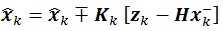
[http://dx.doi.org/10.1007/s10236-003-0036-9] ]. The algorithm assimilates both prediction and measurement by determining which information reflects the actual model. Subsequently, it establishes the weight factors for the two sources of data respectively. In regular Kalman filter method, information from prediction and measurement will be used to govern the estimated value of a particular parameter by the following mathematical representation:
 |
(1) |
 |
(2) |
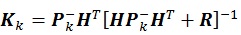
Matrix P-K is the covariance matrix of state parameter, while matrix KK is the Kalman gain which is a matrix that gives weight factor for measurement and prediction data. The variables X-K and Z-K represent information pertained to the parameter x gained from the prediction and measurement data, respectively. Matrix H is called transformation matrix, which is used to transform parameter unit into measurement unit. Matrix R denote the measurement noise that usually generated using standard normal distribution.
The formulation of the regular Kalman filter demonstrated by equations (1) (2) is in the form of linear expression which describes a linear model. On the other hand, history matching analysis encompasses non-linear problem. Hence, regular Kalman filter approach is not suitable to be implemented in this particular case. This issue could be handled by implemented the Ensemble Kalman Filter (EnKF) procedure [17G. Evensen, "Sequential data assimilation with a nonlinear quasi-geostrophic model using monte carlo methods to forecast error statistics", J. Geophys. Res., vol. 99, pp. 10143-10162, 1994.
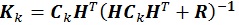
[http://dx.doi.org/10.1029/94JC00572] ]. This technique uses randomization of static parameters as an ensemble and utilizes the ensemble covariance as a representation of the true covariance model. Equation (3) illustrates the mathematical representation for the EnKF which updates the regular Kalman filter formulation as was displayed in equation (2). In this study, we employ the EnKF consideration instead of the regular Kalman filter scheme.
 |
(3) |
Matrix CK is the covariance matrix which is generated by ensemble members. Since initial covariance matrix generates static parameters, it is imperative to ascertain this matrix so that it represents the behavior of the static parameters.
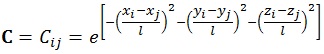
The most crucial static parameters in the history matching study are porosity and permeability. From geological consideration, for instance sedimentation process, it is inferred that porosity and permeability are spatially correlated. Such correlation could be formulated using the Gaussian correlation model [18G. Naevdal, "Reservoir monitoring and continuous model updating using ensemble kalman filter", In: Society of Petroleum Engineers Denver, Colorasdo, USA, 2003, pp. 66-74.] as is shown by the following formulation:
 |
(4) |
The variables x, y, z represent grid numbers in Cartesian axis in x, y, and z direction, respectively. Variable l expresses the correlation length, while the dummy indexes i, j are the grid indexes under corresponding Cartesian axis x, y, and z. The correlation length could be derived from variogram analysis performed during the static modeling process. It can be inferred from equation (4) that adjacent grids will have strongest relationship, illustrated with highest correlation value amongst them. However, the situation will not always follow this basic rule, particularly when the grids are under different region models such as facies, rock type, or flow unit. To address this problem, we modify the Gaussian correlation by introducing matrix modifier term (F) defined as:
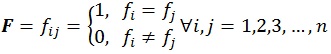 |
(5) |
Where i, j is the grid index while n represents the total grid. Vector f accounts for the region model index that is used in the reservoir model. By incorporating matrix modifier term F, the original Gaussian correlation displayed in equation (4) is modified into the following expression:
 |
(6) |
The matrix multiplication procedure in equation (6) is also known as the Hadamard product. The Schur Product Theorem states that if both F and C are positive semidefinite matrices, then the Hadamard product of them would also be positive semidefinite [19I. Schur, "Bemerkungen zur Theorie der beschränkten Bilinearformen mit unendlich vielen Veränderlichen", In: Journal für die reine und angewandte Mathematik., vol. Vol. 140. Crelle's Journal, 1911, pp. 1-28.]. Meanwhile, there is no guarantee that both F and C and matrices are in positive semidefinite form in our history matching case. To overcome this obstacle, we incorporate two procedures in our algorithm to compute the nearest positive semidefinite matrices. These procedures are based on either Frobenius norm or L2 norm [20N.J. Higham, "Computing a nearest symmetric positive semidefinite matrix", Linear Algebra Appl., pp. 103-118, 1988.
[http://dx.doi.org/10.1016/0024-3795(88)90223-6] ].
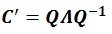
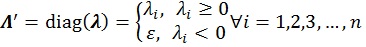
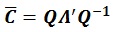
Under Frobenius norm consideration, the existence of a unique solution that is nearest to the matrix C’ can be confirmed by the following equations:
 |
(7) |
 |
(8) |
 |
(9) |
Matrix
 is a diagonal matrix consists of eigenvalues derived from the eigenvalue decomposition, while matrix Q is an eigenvectors matrix. If negative eigenvalues are found during the calculation process, these values will be replaced with the smallest positive real number ɛ. This number is limited by the accuracy of numerical representation in computer memory.
Meanwhile, under the L2 norm, the existence of a solution that is nearest to the matrix C’ can be verified using the following equations:
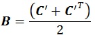 |
(10) |
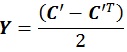 |
(11) |
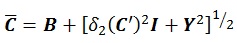 |
(12) |
The challenge in calculating nearest correlation matrix under L2 norm is to determine the value of δ2(C'), which is a L2 norm distance function. Either way, both solutions are adequate to ensure positive definiteness of correlation matrix. It should be noted that although there is a unique solution under Frobenius Norm, there is no guarantee that such unique solution exists under L2 norm [20N.J. Higham, "Computing a nearest symmetric positive semidefinite matrix", Linear Algebra Appl., pp. 103-118, 1988.
[http://dx.doi.org/10.1016/0024-3795(88)90223-6] ]. After correlation matrix is attained, the matrix
 is converted into covariance matrix
 by using standard deviation σ of the static parameters.
 |
(13) |
If every single of static parameters in the grid has their standard deviation, the covariance matrix could be calculated using the following formula:
 |
(14) |
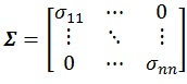 |
(15) |
Matrix Σ is the diagonal matrix which is calculated from standard deviation of the stated parameters. Once the covariance matrix has been obtained, the ensemble could be generated by implementing Cholesky Decomposition into the covariance matrix
, as is exemplified by the following formula:
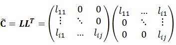 |
(16) |
If the generated covariance matrix is not in positive definite form, the Cholesky Decomposition will fail. Therefore, it is important to find nearest positive definite matrix in the previous step to prevent such problem. Nevertheless, it is important to mention that while there exists unique solution under Frobenius norm realm, there is no guarantee that such unique solution exists under L2 norm [20N.J. Higham, "Computing a nearest symmetric positive semidefinite matrix", Linear Algebra Appl., pp. 103-118, 1988.
[http://dx.doi.org/10.1016/0024-3795(88)90223-6] ].
After triangular matrix L is obtained, the ensemble state parameter X is built using the following equation:
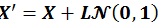 |
(17) |
 |
(18) |
Matrix N (0, 1) is generated from random numbers which is based on standard normal distribution. The resulting ensemble state X' will contain n grid and m realizations of state parameter x.
 |
(19) |
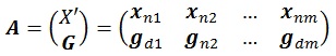
Under EnKF method, for every ensemble member, matrix X' is combined with prediction matrix G Matrix G contains of d prediction and m randomization of vector g.
 |
(20) |
Therefore, the EnKF equation becomes:
 |
(21) |
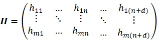
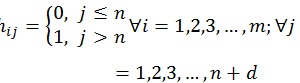
Hence, to calculate Kalman Gain as in equations (3) and (21), the transformation matrix H is needed to transform matrix X' into matrix Xd. The transformation matrix H consists of m times n + d elements, where d denotes the number of measurement vector Z.
 |
(22) |
 |
(23) |
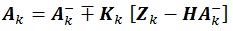
The covariance matrix is updated using the following formula [4G. Evensen, "The ensemble kalman filter: Theoretical formulation and practical implementation", Springer-Verlag Ocean Dyn., vol. 53, pp. 343-367, 2003.
[http://dx.doi.org/10.1007/s10236-003-0036-9] ]:
 |
(24) |
3. VISUALIZATION OF REGION BASED COVARIANCE LOCALIZATION ENKF METHODOLOGY
The previous algorithm could be further explained by an example. All visualization is done by using Matplotlib [21J.D. Hunter, "Matplotlib: A 2D graphics environment", Comput. Sci. Eng., vol. 9, no. 3, pp. 90-95, 2007.
[http://dx.doi.org/10.1109/MCSE.2007.55] ].
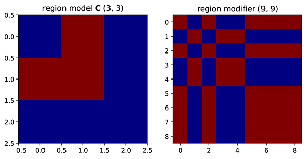 |
Fig. (1) Region model and resulting region modifier. On the region modifier, red represent one while blue represents zero. |
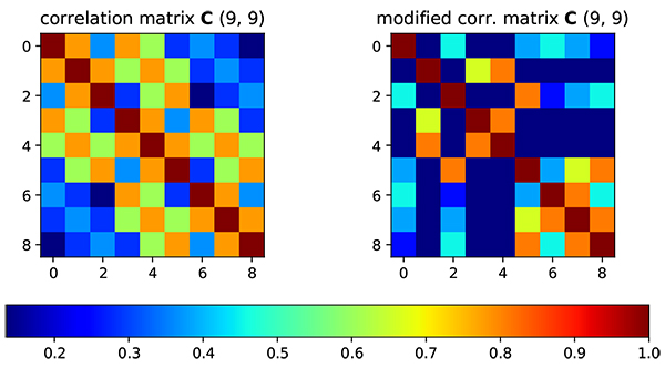 |
Fig. (2) On the left side, correlation matrix is generated by Gaussian correlation model. On the right side, correlation matrix has been modified by region modifier. |
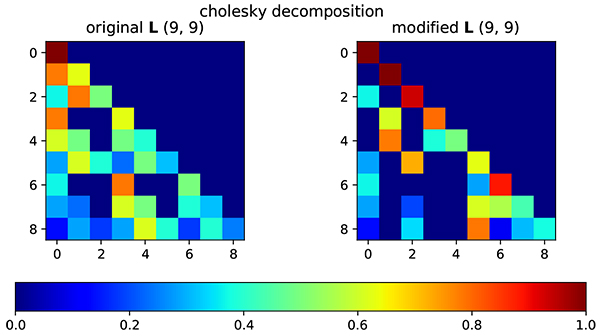 |
Fig. (3) Lower triangular matrix of original correlation matrix (left) and modified correlation matrix (right). |
Suppose there is a region model that represents two facies in the reservoir model as shown in Fig. (1 ). From a geological point of view, the closer the distance between grid the high will be the spatial correlation. However, even if the grid is adjacent, the static parameters on red facies should not be correlated to the blue facies. Therefore, from this rule, we could generate modifier that is based on region information (Fig. 2
 ).
).
The initial correlation matrix is generated using Gaussian correlation model. From color representation, it is clearly shown that the correlation value is decreased when the distance between grid is increased. After correlation matrix is obtained, the correlation matrix is factorized using Cholesky Decomposition as Fig. (3 ).
).
This lower triangular matrix is used to generate correlated random and create ensemble realization of the initial reservoir model. The effect of modified triangular matrix could be seen by generating random data point on a 2D plane as illustrated in Fig. (4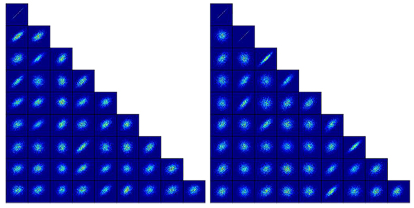 ).
).
 |
Fig. (4) Randomization result based on original lower triangular matrix (left) and modified lower triangular matrix (right). |
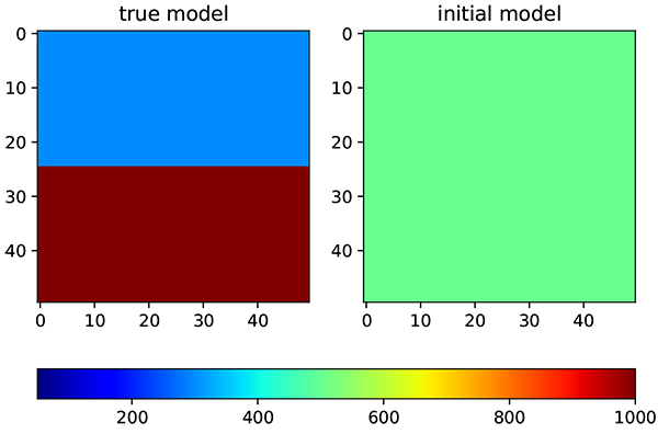 |
Fig. (5) Permeability distribution. On the left is true model while on the right side is initial distribution. |
The randomization result follows the behavior of the pre-determined modifier. It is shown on the map that if there is no correlation, the distribution shape is closer to round.
4. RESULTS OF IMPLEMENTATION OF REGION-BASED COVARIANCE LOCALIZATION ENKF
The synthetic reservoir model is created to test the capability of the region based covariance modifier EnKF to perform history matching. This synthetic reservoir model has two distinct facies with different permeability distribution on each facies (Fig. 5 ).
).
First facies have a permeability of 200 md, while second facies have a permeability of 1000 md. The algorithm will start on an initial model with the permeability of 500 md. The selection of permeability values gives more challenge as the algorithm needs to increase and decrease the permeability distribution in the different part of reservoir model at the same time. Other reservoir parameters are kept the same between true and initial model to prevent bias in the result. The number of well is maintained at a minimum, one well for each facies, to see how far the algorithm could find correct distribution. The distribution is updated by assimilating the prediction from the model and measurement data, in this case, it is an oil production from each well. The reservoir parameters are presented in (Table 1).
The problem initially solved using standard EnKF. Initial ensemble consists of 50 realizations which is generated using equation (17). The correlation matrix is developed using gaussian correlation model to maintain spatial correlation through the ensemble updates. Correlation length used in gaussian correlation model is 500 ft., which equal to 5 grids. The correlation matrix is transformed into covariance matrix by applying eq. (13) using standard deviation of 10% of initial permeability. The average permeability The oil production from all realization and the resulting history match are shown in Figs. (6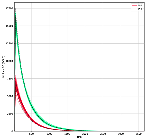 and 7
and 7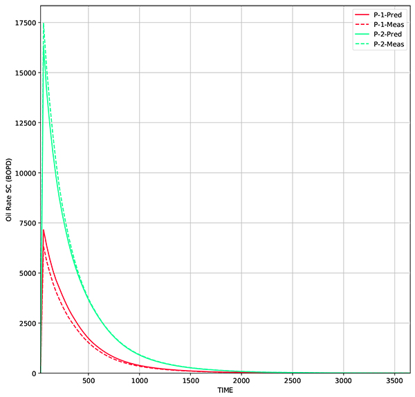 ) while the average permeability from all realizations are shown in Fig. (8
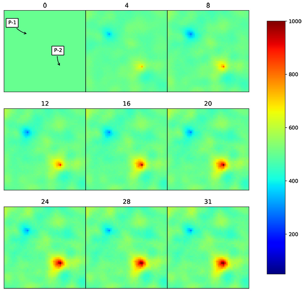 ).
).

 |
Fig. (7) Oil rate from 50 realizations. Solid line represents the oil rate from average permeability, while dashed line represents measurement data. |
 |
Fig. (8) Oil rate from reservoir model that is built using average permeability of all realizations. The updated model gives a production profile that matches to the true model. |
Under EnKF, the updated permeability distribution over time follows the actual model distribution, but only in the area close to the wells. The updated distribution follows spatial correlation that has been defined using Gaussian correlation model. Even though the distribution is still far from the actual model, the production data is already matched. The root mean squared error (RMSE) for the resulting grid is 336 md, while for production data, RMSE for W-1 is 188 BOPD and W-2 is 217 BOPD.
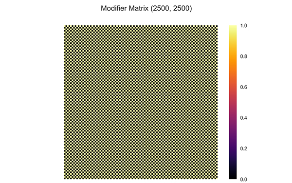 |
Fig. (9) Heatmap of modifier matrix generated by equation (5) for two facies model. The correlation from different facies is removed. |
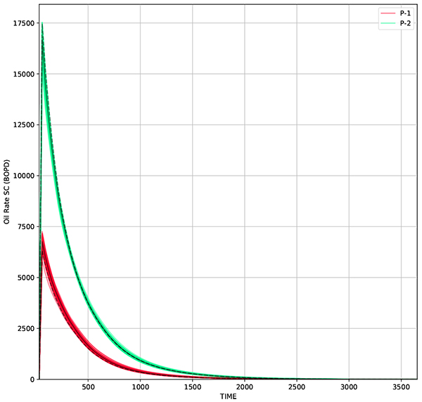 |
Fig. (10) Oil rate from 50 realizations using RCL-EnKF. Solid black line represents oil rate from average permeability, while dashed line represent measurement data. |
It means that the updated grid near the wellbore already gives significant effect to oil production. This outcome confirms that history matching gives a non-unique solution. Under the practical situation, such result could give the wrong impression that the updated distribution already represents accurate reservoir model. Therefore, to minimize the consequence, it is important to add another boundary condition, such as geological or petrophysical information. Updating permeability distribution while maintaining geological or petrophysical model would reduce the probability of non-unique solution.
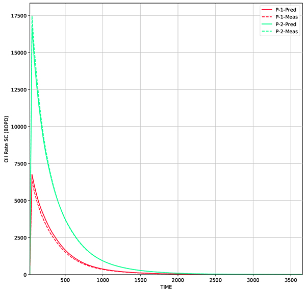 |
Fig. (11) Comparison of oil rate from model generated by RCL-EnKF and true model. The reservoir model is built using average permeability of 50 realizations. |
Using the same parameters, the region based covariance localization EnKF is implemented. RCL-EnKF is implemented by implementing eq. (5) to the correlation matrix generated by gaussian correlation model. To ensure that the modified correlation matrix maintains the positive semidefinite properties, eqs. (7) (8) and (9) are used. The modified correlation matrix is transformed into correlation matrix using eq. (13). Finally, the correlation matrix is used to generate initial ensemble by implementing eqs. (17) and (18). The modifier matrix is shown in (Fig. 9 ).
).
From the snapshot of permeability distribution over time Fig. (12 ) it shows that the facies model is preserved, while updating the permeability distribution. RMSE for the resulting grid is 229 md, while for production data, Figs. (10
 and 11
 ) RMSE for W-1 is 106 BOPD and W-2 is 137 BOPD. The comparison of RMSE for different methods are presented in Table (2). The preservation of facies model gives a real advantage as the updated model does not change the geological concept that has been implemented in the reservoir. Therefore, this algorithm practically can be used in the daily operation in reservoir management workflow.
The estimated permeability distribution is different from true model since the algorithm only assimilates few data, which is single well for each facies. If measurement data is added, the estimated permeability would be much closer to true model. For example, if we add additional wells to the previous model, the permeability RMSE error is reduced into 189.45 md, which makes it closer to true model (Fig. 13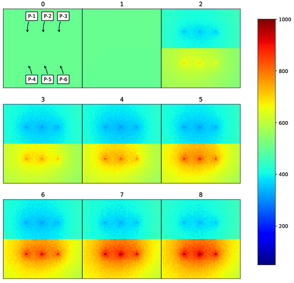 ).
).

To further test this concept, the real facies model is used. The facies model is taken from the geological study of X field in Indonesia, which consists of two distinctive facies (Fig. 14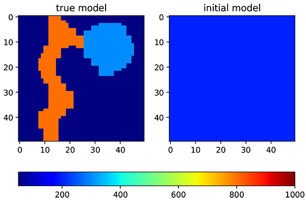 ). The first facies is a channelized reservoir and the second facies is levee area. The permeability of the channel reservoir is substantially higher than in levee area. On the channel area, the average permeability is 800 md, while on the levee area the average permeability is 300 md. The initial input is a homogenous model with permeability of 200 md. There is only three production wells available in the field. Other reservoir and ensemble parameters are kept the same as the previous model to reduce the bias in evaluations.
 |
Fig. (14) Permeability distribution that follows facies model from X field in Indonesia. On the left is a true model, while on the right side is an initial permeability distribution. |
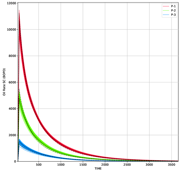 |
Fig. (15) Oil rate from 50 realizations using standard EnKF method. Solid black line represent oil rate from average permeability while dashed line represent measurement data. |
Under such facies model, standard EnKF could give a match results with RMSE of 205 md Figs. (15 and 16
 ). But the resulting permeability distribution is far from true model (Fig. 17
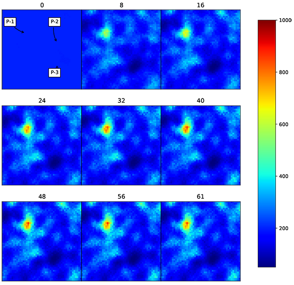 ). The channel reservoir is not well preserved under standard EnKF updating process.
 |
Fig. (16) Comparison of oil rate from true model and predicted model using Standard EnKF. The reservoir model is built using average permeability of 50 realizations. |
 |
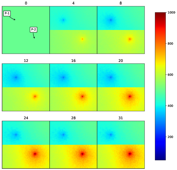
Fig. (17) Change of permeability distribution over time using standard EnKF. The facies model does not follow the facies concept developed by geological study. |
Using the same parameters, the RCL-EnKF is implemented. The modifier matrix is visualized in Fig. (18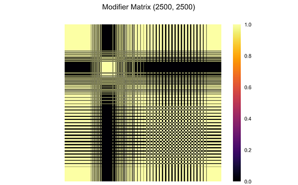 ). The result shows that the predictions are matched to the measurement data (Figs. 19 and 20
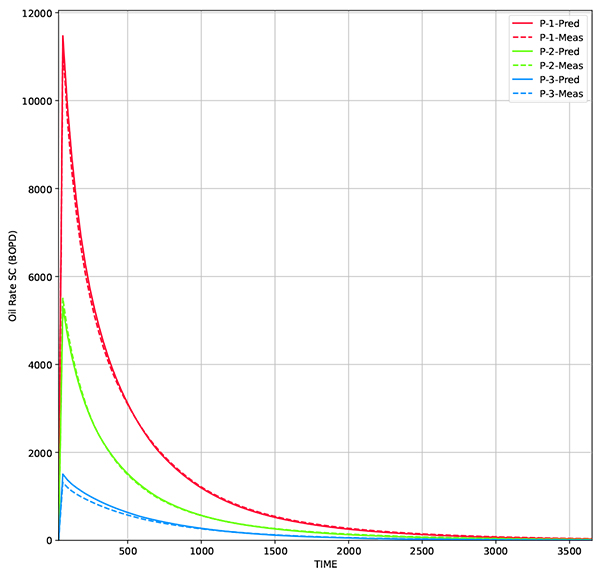 ). The permeability distribution is updated, while following designated facies model, resulting in more accurate results (Fig. 21
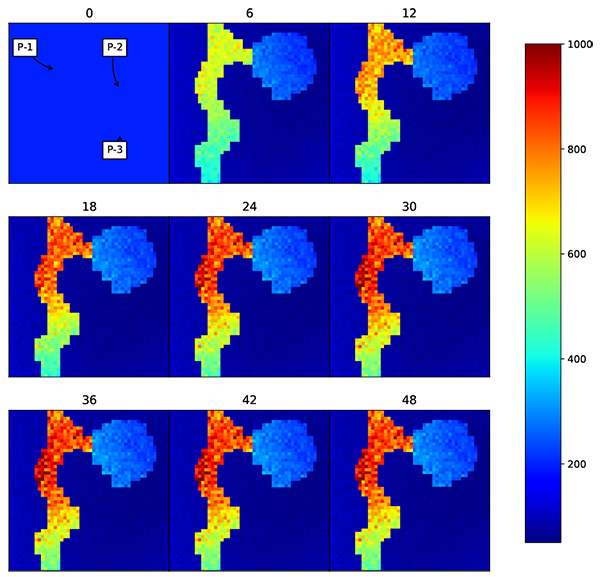 ). Also in this scenario, RCL-EnKF method reducing the grid RMS error from 205 md to 42 md, which is 79% error reduction (Table 3).
 |
Fig. (18) Heatmap of modifier matrix generated by equation (5) for channelized facies model. The correlation from different facies is removed. |
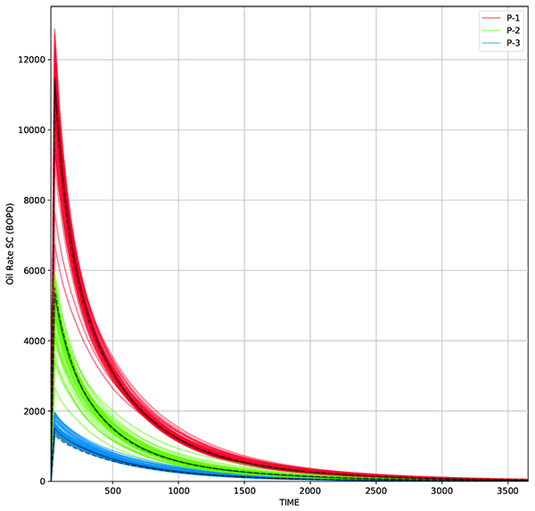 |
Fig. (19) Oil rate from 50 realizations using RCL-EnKF method. Solid black line represent oil rate from average permeability while dashed line represent measurement data. |
 |
Fig. (20) Comparison of oil rate from true model and predicted model using RCL-EnKF. The reservoir model is built using average permeability of 50 realizations. |
 |
Fig. (21) Change of permeability using RCL EnKF. The facies model is preserved while updating the permeability values. |
CONCLUSION
Implementation of region based covariance localization in EnKF has successfully updated the parameter distribution by incorporating parameter modification process within a region model. Hence, the generated parameter distribution should be able to maintain the geological or petrophysical notions. This endeavor enables geological justification for the generated parameter distribution. The RMSE error for RCL-EnKF is considerably lower than standard EnKF. The algorithm is relatively straightforward, hence suitable to be applied in reservoir management workflow.
The RCL-EnKF is highly dependent on the quality of facies estimation. Having good estimate of facies model will gives accurate results. Usually in early development of reservoir, the estimated facies model has high uncertainty. This could introduce bias in updating process. To improve the quality of reservoir properties estimation, this method could be combined with another EnKF based facies prediction method [18G. Naevdal, "Reservoir monitoring and continuous model updating using ensemble kalman filter", In: Society of Petroleum Engineers Denver, Colorasdo, USA, 2003, pp. 66-74.]. The facies are predicted prior to reservoir properties estimation.
Another challenge is if there is too many facies type in the model, it is possible to produce matched results yet inaccurate properties distribution due to increased degree of freedom. Adding limit on EnKF search space could potentially reduce the degree of freedom and improve the results.
The proposed localization method is not limited only to EnKF. Implementation of region based covariance localization on another algorithm is yet to be investigated. The proposed localization could possibly be used to test the consistency of seismic inversion with the prior facies model by evaluating elastic model parameters.
CONSENT FOR PUBLICATION
Not applicable.
CONFLICT OF INTEREST
The authors declare no conflict of interest, financial or otherwise.
ACKNOWLEDGEMENTS
Our sincere thanks to Computer Modeling Group for their donation of simulator licenses to Institut Teknologi Bandung, and to SKK Migas for providing facies model data. The authors would also like to acknowledge the help of Aditya Dewanto Hartono from Kyushu University in reviewing this paper.
REFRENCES
| [1] | Z. Tavassoli, J.N. Carter, and P.R. King, "Errors in history matching", SPE J., pp. 352-361, 2004. [http://dx.doi.org/10.2118/86883-PA] |
| [2] | Z. Ji, and M. Brown, "Joint state and parameter estimation for biochemical dynamic pathways with iterative extended kalman filter: Comparison with dual state and parameter estimation", Open Auto. and Cont. Sys., vol. 2, pp. 69-77, 2009. [http://dx.doi.org/10.2174/1874444300902010069] |
| [3] | G. Everson, "Advanced data assimilation for strongly nonlinear dynamics", Mon. Weather Rev., vol. 125, no. 6, pp. 1342-1354, 1997. [http://dx.doi.org/10.1175/1520-0493(1997)125<1342:ADAFSN>2.0.CO;2] |
| [4] | G. Evensen, "The ensemble kalman filter: Theoretical formulation and practical implementation", Springer-Verlag Ocean Dyn., vol. 53, pp. 343-367, 2003. [http://dx.doi.org/10.1007/s10236-003-0036-9] |
| [5] | G. Eversen, "Sampling strategies and square root analysis schemes for EnKF", Ocean Dyn., vol. 54, pp. 539-560, 2004. [http://dx.doi.org/10.1007/s10236-004-0099-2] |
| [6] | H.L. Mitchell, and P.L. Houtekamer, "Data assimilation using an ensemble kalman filter technique", Mon. Weather Rev., vol. 126, pp. 796-811, 1998. [http://dx.doi.org/10.1175/1520-0493(1998)126<0796:DAUAEK>2.0.CO;2] |
| [7] | A. Bianco, A. Cominelli, L. Dovera, G. Naevdal, and B. Valles, "History Matching and Production Forecast Uncertainty by Means of the Ensemble Kalman Filter: A Real Field Application", In: SPE Europec/EAGE Annual Conference and Exhibition, London, 2007. [http://dx.doi.org/10.2118/107161-MS] |
| [8] | V. Haugen, G. Naevdal, L.J. Natvik, G. Evensen, A.M. Berg, and K.M. Flornes, "History matching using the ensemble kalman filter on a north sea field case", SPE J., pp. 382-391, 2008. [http://dx.doi.org/10.2118/102430-PA] |
| [9] | M. Zafari, and A. Reynolds, "Assessing the uncertainty in reservoir description and performance predictions with the ensemble kalman filter", SPE Annual Technical Conference and Exhibition, Dallas, 2005. [http://dx.doi.org/10.2118/95750-MS] |
| [10] | T.M. Hamill, and J.S. Whitaker, "Distance-dependent filtering of background error covariance estimates in an ensemble kalman filter", Mon. Weather Rev., vol. 129, pp. 2776-2790, 2001. [http://dx.doi.org/10.1175/1520-0493(2001)129<2776:DDFOBE>2.0.CO;2] |
| [11] | Y. Chen, and D.S. Oliver, "Cross-covariances and localization for EnKF in multiphase flow data assimilation", Computat. Geosci., vol. 14, no. 4, pp. 579-601, 2010. [http://dx.doi.org/10.1007/s10596-009-9174-6] |
| [12] | D. Devegowda, "Streamline Assisted Ensemble Kalman Filter", Formulation & paid application, Texas A&M University: College Station, Texas Tx, USA, 2009. |
| [13] | A. Datta-Gupta, and M.J. King, Streamline Simulation: Theory and Practice, Richardson: SPE Textbook Series #11, 2007. |
| [14] | A.A. Emerick, and A.C. Reynolds, "History Matching a Field Case Using the Ensemble Kalman Filter with Covariance Localization", SPE Reservoir Simulation Symposium, Woodlands, Taxas, 2011. [http://dx.doi.org/10.2118/141216-MS] |
| [15] | X. Luo, T. Bhakta, and G. Nædal, "Data driven adaptive localization with applications to ensemble-based 4D seismic history matching", SPE Bergen One Day Seminar, Bergen, 2017. [http://dx.doi.org/10.2118/185936-MS] |
| [16] | Y. Zhao, A.C. Reynolds, and G. Li, "Generating facies maps by assimilating production data and seismic data with the ensemble kalman filter", SPE/DOE Improved Oil Recovery Symposium, Tulsa, 2008. [http://dx.doi.org/10.2118/113990-MS] |
| [17] | G. Evensen, "Sequential data assimilation with a nonlinear quasi-geostrophic model using monte carlo methods to forecast error statistics", J. Geophys. Res., vol. 99, pp. 10143-10162, 1994. [http://dx.doi.org/10.1029/94JC00572] |
| [18] | G. Naevdal, "Reservoir monitoring and continuous model updating using ensemble kalman filter", In: Society of Petroleum Engineers Denver, Colorasdo, USA, 2003, pp. 66-74. |
| [19] | I. Schur, "Bemerkungen zur Theorie der beschränkten Bilinearformen mit unendlich vielen Veränderlichen", In: Journal für die reine und angewandte Mathematik., vol. Vol. 140. Crelle's Journal, 1911, pp. 1-28. |
| [20] | N.J. Higham, "Computing a nearest symmetric positive semidefinite matrix", Linear Algebra Appl., pp. 103-118, 1988. [http://dx.doi.org/10.1016/0024-3795(88)90223-6] |
| [21] | J.D. Hunter, "Matplotlib: A 2D graphics environment", Comput. Sci. Eng., vol. 9, no. 3, pp. 90-95, 2007. [http://dx.doi.org/10.1109/MCSE.2007.55] |