- Home
- About Journals
-
Information for Authors/ReviewersEditorial Policies
Publication Fee
Publication Cycle - Process Flowchart
Online Manuscript Submission and Tracking System
Publishing Ethics and Rectitude
Authorship
Author Benefits
Reviewer Guidelines
Guest Editor Guidelines
Peer Review Workflow
Quick Track Option
Copyediting Services
Bentham Open Membership
Bentham Open Advisory Board
Archiving Policies
Fabricating and Stating False Information
Post Publication Discussions and Corrections
Editorial Management
Advertise With Us
Funding Agencies
Rate List
Kudos
General FAQs
Special Fee Waivers and Discounts
- Contact
- Help
- About Us
- Search


The Open Petroleum Engineering Journal
(Discontinued)
ISSN: 1874-8341 ― Volume 12, 2019
Investigating the Effect of Interlayer Geo-stress Difference on Hydraulic Fracture Propagation: Physical Modeling and Numerical Simulations
Xiaosen Shang1, 2, *, Yunhong Ding2, Lifeng Yang2, Yonghui Wang2, Tao Wang3
Abstract
The morphological control of the fracture has a great impact on the effectiveness of the hydraulic fracturing; the geostress difference between productive interval and barriers is one of controlling factors for the fracture height control. The propagation behavior of the hydraulic fracture was studied using the 3D physical simulation under conditions of the presence and absence of the interlaminar geostress difference. Combined with the result of the acoustic monitoring, the dynamic propagation process and the final shape of fracture were achieved. It shows that the lateral and vertical propagations of the fracture simultaneously occurred without the interlaminar geostress difference, and a fracture with round-shape face was finally presented. On the contrary, under the presence of the interlaminar geostress difference, due to the barrier effect of the high stress barrier on the vertical propagation of the fracture, the fracture height was obviously limited after the fracture propagated to the interval boundary. Therefore, the final shape of the fracture face was elliptical. Moreover, the extended finite element simulation was also adopted to analyze the propagation of the hydraulic fracture under two conditions mentioned above, and the result was consistent with that of the physical simulation. This verifies the feasibility of the extended finite element simulation method; therefore, this method was used to further simulate the fracture propagation behavior when several layers with different stiffness simultaneously exist. The result presents that during the fracture propagation, the fracture passed through the layer which has relatively weak stiffness and stopped before the layer which has stronger stiffness. Conclusions of this study can provide reference for the research of fracture propagation in complex geostress reservoirs.
Article Information

Identifiers and Pagination:
Year: 2016Volume: 9
First Page: 195
Last Page: 206
Publisher Id: TOPEJ-9-195
DOI: 10.2174/1874834101609160195
Article History:
Received Date: 14/12/2015Revision Received Date: 18/02/2016
Acceptance Date: 19/04/2016
Electronic publication date: 29/08/2016
Collection year: 2016
open-access license: This is an open access article licensed under the terms of the Creative Commons Attribution-Non-Commercial 4.0 International Public License (CC BY-NC 4.0) (https://creativecommons.org/licenses/by-nc/4.0/legalcode), which permits unrestricted, non-commercial use, distribution and reproduction in any medium, provided the work is properly cited.
* Address correspondence to these authors at the China University of Petroleum (East China), Qingdao, 266580, P.R. China; Tel: +86-010 8359 5362; E-mail: shangxs521@163.com
| Open Peer Review Details | |||
|---|---|---|---|
| Manuscript submitted on 14-12-2015 |
Original Manuscript | Investigating the Effect of Interlayer Geo-stress Difference on Hydraulic Fracture Propagation: Physical Modeling and Numerical Simulations | |
1. INTRODUCTION
Hydraulic fracturing is one of the key techniques to develop the ultra-low permeability or unconventional oil or gas reservoirs. It has been widely used to enlarge the seepage area of oil and gas, to change the flow pattern of oil and gas, and to allete the bottom hole contamination to improve the well production [1C.L. Cipolla, N.R. Warpinski, M.J. Mayerhofer, E.P. Lolon, and M.C. Vincent, The relationship between fracture complexity, reservoir properties, and fracture-treatment design, SPE Annual Technical Conference and Exhibition, 21-24 September 2010, Denver, Colorado.
[http://dx.doi.org/10.2118/115769-PA] , 2W. Kan, and E.O. Jon, "Mechanics analysis of interaction between hydraulic and natural frsctures in shale reservoirs", In: Unconventional Resources Technology Conference, 25-27 August 2014 Denver, Colorado.]. Morphological control of the hydraulic fracture, especially the height control of fracture, has a great impact on the effectiveness of hydraulic fracturing [3H.R. Gu, and E. Siebrits, "Effect of formation modulus contrast on hydraulic fracture height containment", SPE J., vol. 23, pp. 170-176, 2006.]. When the hydraulic fracture extends beyond the productive layer, it may communicate the above and below layers with the productive area. The unblocking of the local aquifers gushing into the wellbore through the hydraulic fracture may lead to the failure of hydraulic fracturing [4G.M. Gou, and R.Q. Hu, "Controlling gap height and fracture to thin layer", Well Test, vol. 13, pp. 48-53, 2004.].
Many influencing factors can affect the control behavior of fracture height. Lian [5P.Q. Lian, L.S. Cheng, and B. Deng, "Simulation of ground stress field and fracture anticipation with effect of pore pressure", Theor. Appl. Fract. Mech., vol. 56, pp. 34-41, 2011.
[http://dx.doi.org/10.1016/j.tafmec.2011.09.004] ], Mohammad [6J.N. Mohammad, and M. Ali, "Effects of in-situ stress regime and intact rock strength parameters on the hydraulic fracturing", J. Petrol. Sci. Eng., vol. 108, pp. 211-221, 2013.
[http://dx.doi.org/10.1016/j.petrol.2013.04.001] ] and Gou [4G.M. Gou, and R.Q. Hu, "Controlling gap height and fracture to thin layer", Well Test, vol. 13, pp. 48-53, 2004.] have studied several influencing factors on the fracture control, such as the properties of the barriers, variations in fracture opening moduli, stress field, and additional stresses due to leak-off, as well as some strategies were discussed. Geostress difference between the productive interval and barriers is one of the key controlling factors for the fracture height control. Gudmundsson [7G. Agust, H.S. Trine, L. Belinda, and L.P. Sonja, "Effects of internal structure and local stresses on fracture propagation, deflection, and arrest in fault zones", J. Struct. Geol., vol. 32, pp. 1643-1655, 2010.
[http://dx.doi.org/10.1016/j.jsg.2009.08.013] ] found that fractures tended to torture or stop before the contact of layers with different stiffness. Compared to the extension from the soft layer to the stiff layer, the fracture propagation from the opposite direction was easier to happen. Adachi [8I.A. Jose, D. Emmanuel, and P.P. Anthony, "Analysis of classical pseudo-3D model for hydraulic fracture with equilibrium height growth across stress barriers", Int. J. Rock Mech. Min. Sci., vol. 47, pp. 625-639, 2010.
[http://dx.doi.org/10.1016/j.ijrmms.2010.03.008] ], Chitrala [9C. Yashwanth, M. Camilo, S. Carl, and R. Chandra, "An experiment investigation into hydraulic fracture propagation under different applied sresses in tight sands using acostic emissions", J. Petrol. Sci. Eng., vol. 108, pp. 151-161, 2013.
[http://dx.doi.org/10.1016/j.petrol.2013.01.002] ], Warpinski [10N.R. Warpinski, J.A. Clark, R.A. Schmidt, and C.W. Huddle, "Laboratory investigation on the effect of In situ stresses on hydraulic fracture containment", SPE J., vol. 22, pp. 333-340, 1982.
[http://dx.doi.org/10.2118/9834-PA] ] and Teufel [11L.W. Teufel, and J.A. Clark, "Hydraulic fracture propagation in layered rock: experimental studies of fracture containment", SPE J., vol. 24, pp. 19-32, 1984.
[http://dx.doi.org/10.2118/9878-PA] ] investigated the influence of stress on fracture propagation through theoretical and experimental methods, respectively. The barrier effect on fracture height growth was clear in the cases that high stress was given to the formation. Guo [12T.K. Guo, S.C. Zhang, Z.Q. Qu, T. Zhou, Y.S. Xiao, and J. Gao, "Experimental study of hydraulic fracturing for shale by stimulated reservoir volume", Fuel, vol. 128, pp. 373-380, 2014.
[http://dx.doi.org/10.1016/j.fuel.2014.03.029] ] and Li [13Y.P. Li, Y.H. Wang, Y.H. Ding, X. Wang, and L.F. Yang, "Physical and Numerical Simulation of Hydraulic Fracture Initiation and Propagation in Gas Shale", In: SPE Unconventional Resources Conference and Exhibition-Asia Pacific., 11-13 November 2013 Brisbane, Australia,.] studied the hydraulic fracture propagation in shale which has the structure of weak planes and natural fractures by experiment; they also investigated the final fracture morphology using CT scanning and found that some natural fractures or sedimentary beddings were opened and some of them could stop the growth of induced fractures.
In the numerical study of fracture propagation, many methods including the extended finite element method, the boundary element method, the unconventional fracture model, and the discrete fracture network were applied to predict the propagation behavior of the hydraulic fracture [14T. Mohammadnejad, and A.R. Khoei, "An extended finite element method for hydraulic fracture propagation in deformable porous media with the cohesive crack model", Finite Elem. Anal. Des., vol. 73, pp. 77-95, 2013.
[http://dx.doi.org/10.1016/j.finel.2013.05.005] -16J. Oliver, I. Dias, and A.E. Huespe, "Crack-path field and strain-injection techniques in computational modeling of propagating material failure", Comput. Methods Appl. Mech. Eng., vol. 274, pp. 289-348, 2014.
[http://dx.doi.org/10.1016/j.cma.2014.01.008] ]. The extended finite element method allows for a static mesh as fractures extend, and eliminates the need and computational expense of remeshing [17T.S. Jaber, "Numerical modeling of hydraulic fracture propagation: Accounting for the effect of stresses on the interaction between hydraulic and parallel natural fractures", Egypt. J. Pet, vol. 22, pp. 557-563, 2013.
[http://dx.doi.org/10.1016/j.ejpe.2013.11.010] ]. With the application of the extended finite element method, Jaber [17T.S. Jaber, "Numerical modeling of hydraulic fracture propagation: Accounting for the effect of stresses on the interaction between hydraulic and parallel natural fractures", Egypt. J. Pet, vol. 22, pp. 557-563, 2013.
[http://dx.doi.org/10.1016/j.ejpe.2013.11.010] ] discussed the effect of in situ stress anisotropy on fractures interaction, and he concluded that the direction of in situ stresses with respect to natural fractures set was an important factor dominating the efficiency of fracturing treatment. With the development of unconventional reservoirs, the hydraulic fracturing technology and fracture propagation behavior are attracting more and more public attention due to the uncertain effectiveness of fracturing [18G.E. King, "Thirty years of gas shale fracturing: what have we learned?", In: SPE Annual Technical Conference and Exhibition, 19-22 September 2010 Florence, Italy.
[http://dx.doi.org/10.2118/133456-MS] ]. Because of the complexity reservoir conditions, different geostress should be considered, especially the interlaminer geostress difference. In this research, we investigated the influence of interlaminer geostress difference on fracture growth behavior using experimental and numerical methods, which can testify effectiveness of the numerical method. Moreover, the fracture propagation when several special layers with different stiffness simultaneously exist was simulated with the application of a horizontal well model. The study can provide reference for the research of fracture propagation in complex stress reservoirs, such as the shale gas reservoir.
2. PHYSICAL SIMULATION SECTION
2.1. Apparatus and Specimen Processing
Physical simulation experiments were conducted in a triaxial hydraulic fracturing physical simulation system, which is shown in the Fig. (1a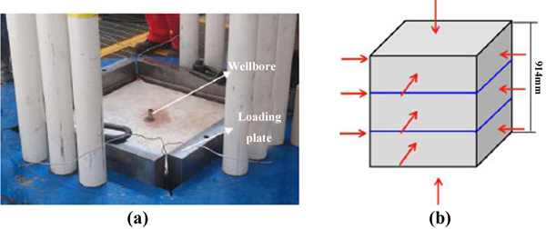 ). A triaxial stress loading system with a function of triaxial loading and rock samples were used in the physical simulation system. The stress loading system is composed of several loading plates and flatjacks which can exert stress on the top and sides of the rock sample. The flatjack used to load horizontal stress consists of three parts and it can exert different stresses on one side of rock, as shown in the Fig. (1b). Acoustic monitoring system was also applied to monitor the dynamic propagation process of the fracture and it could exhibit the distribution of acoustic emission points.
 |
Fig. (1) Schematic of hydraulic fracturing model. (a) picture of triaxial experiment apparatus; (b) schematic of stress loading. |
The rock samples were collected from Changqing oilfield of China, and they have been processed into 762 mm×762 mm×914 mm cubes before experiments. The size of the rock sample is large enough to guarantee that sufficient amount of data can be collected during experiments of actual fracture extension [12T.K. Guo, S.C. Zhang, Z.Q. Qu, T. Zhou, Y.S. Xiao, and J. Gao, "Experimental study of hydraulic fracturing for shale by stimulated reservoir volume", Fuel, vol. 128, pp. 373-380, 2014.
[http://dx.doi.org/10.1016/j.fuel.2014.03.029] ]. An artificial wellbore with an open hole located at the bottom was drilled in the rock sample, as shown in the Fig. (2a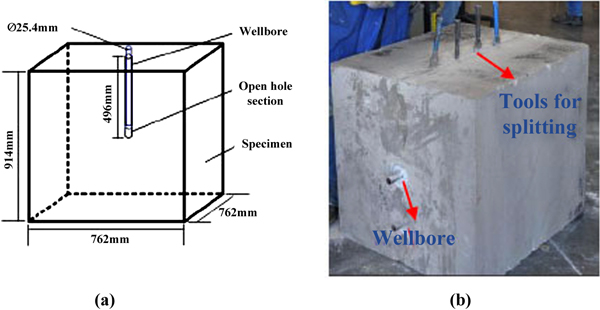 ). The fracturing fluid used in experiments was guar gum fracturing fluid which was colored into red so that the fracture morphology can be presented clearly. It was injected into the open hole with an injection rate of 60mL/min to simulate the actual fracturing process. After the physical simulation experiment, to directly observe the hydraulic fracture, the rock sample was split or cut into pieces to reveal the fracture morphology, as shown in the Fig. (2b).
 |
Fig. (2) Schematic of rock sample processing. (a) rock sample with wellbore; (b)rock sample was split. |
2.2. Procedure
To compare the results of simulations under two conditions of presence and absence of interlaminar geostress difference, two cases are studied: exerting same and different stresses on sides of rock samples. The two rock samples used in two cases have close mechanical parameters and were loaded different stress conditions, as shown in Table. 1. The vertical stress was 20 MPa. The interlaminar geostress difference was considered in the case 2 with the 2# rock sample, and the upper and bottom layers had relatively high geostresses than that of the middle layer.
3. NUMERICAL SIMULATION SECTION
The extended finite element method was applied to conduct the numerical simulation of hydraulic fracture propagation [14T. Mohammadnejad, and A.R. Khoei, "An extended finite element method for hydraulic fracture propagation in deformable porous media with the cohesive crack model", Finite Elem. Anal. Des., vol. 73, pp. 77-95, 2013.
[http://dx.doi.org/10.1016/j.finel.2013.05.005] ]. On the basis of ABAQUS, an explicit user unit subprogram is developed to complete the numerical simulation study. The phantom node method was used to simulate discontinuous displacement in the fracture propagation without changing the basic elements. Thus, the discontinuity can be realized on the basis of the finite element program. As to the integration process, a virtual velocity was applied to control the occurrence of hourglass, which may be induced by reduced integration. In addition, the finite difference method was applied on the controlling equations of fluid, and the leak off of fracturing fluid from fracture to matrix was not considered in the simulations. The numerical modeling is single-phase. The dimension of fracture used in the fluid calculation was from the computation of solid failure, and the pressure distribution from fluid calculation was used in the computation of solid failure in the next step.
The criterion for fracture initiation is based on the maximum principal strain. The critical strain used in the simulations were 0.0008. It means that the fracture was initiated when the principal strain become larger than the critical strain:
ε ≥ εc
The classical models of PKN and KGD are 2D models used to describe the fracture growth with some assumptions [19J. Adachi, E. Siebrits, A. Peirce, and J. Desroches, "Computer simulation of hydraulic fractures", Int. J. Rock Mech. Min. Sci., vol. 44, pp. 739-757, 2007.
[http://dx.doi.org/10.1016/j.ijrmms.2006.11.006] ]. Compared with PKN and KGD models, the fracture height in this study varies in the direction of length during the propagation. The fluid flow assumption of laminar flow from wellbore to fracture tip is the same as the assumption in PKN model. As with the PKN model, the vertical cross-section of fracture is elliptical.
According to the similarity, a simulation model (Fig. 3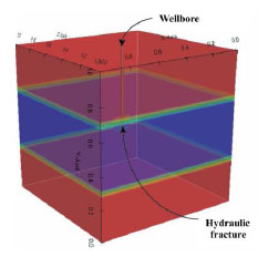 ) was built based on the rock sample used in the physical simulation. It had the size of 1 000 mm×1 000 mm×1 000 mm and was exerted external stress (σv = 20MPa; σh=15MPa; σH = 12MPa). Three layers in this model were also separated and could been given same or different parameter values.
 |
Fig. (3) Schematic of the numerical model. |
The relationship between Young’s modulus and confining stress was obtained from the compressive stiffness test of rock sample, and data are shown in Fig. (4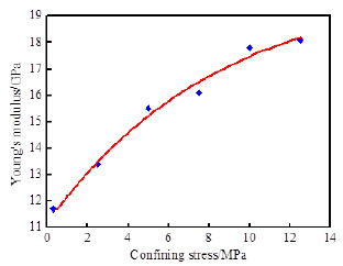 ). It can be seen that the Young’s modulus increases with the increase of the confining stress. According to this kind of monotone increasing trend, the Young’s modulus can be used in the numerical simulation to replace the confining stress, and meanwhile a similar effect can be achieved.
 |
Fig. (4) The relationship between Young’s modulus and confining stress. |
Like the physical simulations, two groups of numerical simulations were conducted, including the propagation of fracture with and without the interlaminar geostress difference.
4. RESULTS AND DISCUSSION
4.1. Fracture Propagation without Interlaminar Geostress Difference
4.1.1. Physical Simulation
This section is on the basis of 1# rock sample. The vertical stress which was exerted on the rock was 20 MPa, and the maximum and minimum horizontal stresses forced on the rock were 8 and 5 MPa, respectively. During the physical simulation process of 1# rock sample, due to that the horizontal stress exerted on the rock sample did not change along the vertical direction, the interlaminar geostress difference was not considered.
After the completion of the hydraulic fracturing experiment, 1# rock sample was taken out of the stress loading system and was split along the propagation direction of the hydraulic fracture so that the fracture face could be revealed. Because the fracturing fluid was colored into red before, the red area on the rock split face was the fracture face area (propagation area), just as shown in the Fig. (5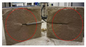 ). It can be found that the fracture face was round when the interlaminar geostress difference did not exist, and a symmetrical double-wing fracture whose propagation direction was perpendicular to the minimum horizontal stress σh was generated.
 |
Fig. (5) Hydraulic fracture face after the hydraulic fracturing. |
Different fracture propagation processes lead to different acoustic emission events [9C. Yashwanth, M. Camilo, S. Carl, and R. Chandra, "An experiment investigation into hydraulic fracture propagation under different applied sresses in tight sands using acostic emissions", J. Petrol. Sci. Eng., vol. 108, pp. 151-161, 2013.
[http://dx.doi.org/10.1016/j.petrol.2013.01.002] ]. Fig. (6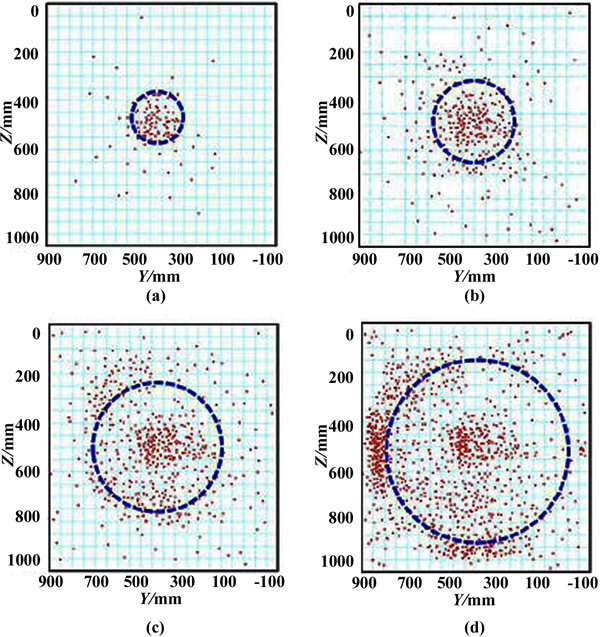 ) presents the distribution of acoustic emission points at different stages of physical simulation, which can present the dynamic propagation process of the fracture. The dimensions here is the dimension used to process the acoustic emission points. It is larger than the dimension mentioned in the text, because the acoustic emission points appear not only within the rock volume but out of the rock when some noises happened there.
 |
Fig. (6) Acoustic emission points distribution at different stages. (a) 400s; (b) 960s; (c) 2200s; (d)3240s. |
It can be found that more acoustic emission points generated with the continuance of the hydraulic fracturing simulation. When the physical simulation time was 400s, because of the relatively short time, acoustic emission points emerged intensively in the location of open hole section of wellbore, just as shown in the Fig. (6a), and it shows the initiation of the hydraulic fracture. With the extension of experimental time to 960 and 2200s, the amount of acoustic emission points intensively increased as shown in Fig. (6b and c), and they present that the fracture gradually propagated. With a further extension of experimental time to 3240s, large numbers of acoustic emission points emerged at the edge of the rock as shown in the Fig. (6d). It could be inferred that the fracture fluid flowed out of the rock sample and the fracture reached the edge of the rock. According to the distribution change of acoustic emission points, it can be found that the lateral and vertical propagation of the fracture occurred, and finally a fracture with round-shape face was formed. It is due to the reason that without the interlaminar geostress difference, no barrier effect existed in the vertical direction, and then the fracture morphology was only controlled by the three-dimension principles stress condition.
4.1.2. Numerical Simulation
In the numerical simulation study, the first group simulation was conducted to investigate the fracture propagation behavior when the interlaminar geostress difference did not exist. In order to simulate the absence of interlaminar geostress difference condition, three layers in the numerical model (Fig. 3) were given a same Young’s modulus value (upper = middle = bottom = 15 GPa). Fig. (7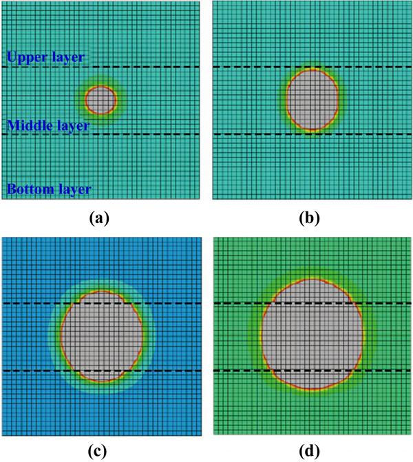 ) shows the result of the numerical simulation with presentation of the change in fracture face. It shows from the Fig. (7a) that when the simulation time was 0.5 ms, the fracture face was relatively small and presented a round shape. With the increase of the simulation time from 0.5ms to 1.2 and 1.6ms, the fracture face was obviously enlarged; however, both of their shapes (Fig. 7b and c) were also round despite that the fracture has already reached and crossed the boundaries of the middle layer. Fig. (7d) illustrates that with the extension of the simulation time to 2.5ms, the fracture further propagated into the upper and bottom layers and the fracture face also showed the round shape. The result of the numerical simulation matched very well with that of the physical simulation.
 |
Fig. (7) Fracture propagation in the first group numerical simulation. (a) 0.5ms; (b)1.2ms;(c) 1.6ms; (d)2.5ms. |
4.2. Fracture Propagation with Interlaminar Geostress Difference
4.2.1. Physical Simulation
The 2# rock sample was used to conduct the physical simulation test when the interlaminar geostress difference was considered. The vertical stress exerted on the 2# rock sample was 20 MPa which was same with that of the 1# rock sample. The horizontal stress exerted on the rock sides changed along the vertical direction. The upper and bottom layers were exerted relatively high horizontal stresses (σH = 15 MPa, σh = 12 MPa), and the middle layer was exerted relatively low stresses (σH = 8 MPa, σh = 5 MPa).
After the physical simulation was performed, the rocksample was cut into slices along the horizontal direction parallel to the fracture face, and then the cross sections of hydraulic fracture in different locations were obtained, just as shown in the Fig. (8 ).
).

Fig. (8a) is the picture of rock slices, and the trace lines on different slices reflected the propagation size of the fracture. That is to say, each slice can be perceived to be one cross section of the hydraulic fracture. The length of the line equals the height of the fracture in the certain location of that slice. In order to describe the fracture more specifically, a schematic was drawn as shown in the Fig. (8b). The blue lines represent the cross sections of fracture in different propagation locations along the horizontal direction, and the red line represents the fracture edge. Note that the Fig. (8) just presents one half of the hydraulic fracture. It can be clearly seen that the larger the distance from the wellbore, the smaller the fracture height, and then an elliptical fracture face was finally achieved.
Fig. (9 ) illustrates the acoustic emission points distribution at several stages of the physical simulation of 2# rock sample. When the simulation time was 440s, points were confined to an area close to the open hole section of wellbore, as shown in the Fig. (9a), and the shape of the area was nearly round. It was due to that the fracture did not reach the boundary of the middle layer at that time. When the physical simulation time was extended to 920s, a large amount of acoustic emission points appeared and located near the boundary of the middle layer (Fig. 9b). It can be inferred that the fracture may reach the boundary. With the increase of the simulation time to 1800s, numbers of points occurred at the right and left parts of the middle layer; however, only a few points appeared at the upper and bottom layers (Fig. 9c). This phenomenon presents that the fracture mainly propagated in the middle layer, and its propagation along the vertical direction was limited by the upper and bottom layers with relatively high stress. From (Fig. 9b and c), more points emerge at the left part than at the right part, and it indicates that the fracture propagation may be not uniform. It may go to the left first then the right, which has no influence on the final shape of the fracture. Fig. (9d) shows the result that at the final time of 2800s, the vast majority of points appeared at the edges of middle layer, and it illustrates that the fracture reached the edge of the rock sample, and the fluid flowed out of the rock. It can be concluded from the above results that with the presence of the interlaminar geostress difference, the fracture height was obviously limited due to the barrier effect of the high stress barriers, and the final shape of the fracture face was elliptical.
 |
Fig. (9) Acoustic emission points distribution at different simulation stages (2# rock). (a) 440s; (b) 920s; (c) 1800s; (d) 2800s. |
4.2.2. Numerical Simulation
In the numerical simulation of the fracture propagation in layers with different interlaminar geostresses, three layers were separated and given different Young’s modulus values (upper: 30GPa; middle: 15GPa; bottom: 30GPa) in the numerical model as shown in the Fig. (3). Similarly, the upper layer and bottom layer were given relative high value than that of the middle layer, and then the influence of geostress difference on the fracture propagation was simulated. The simulation result is shown in Fig. (10 ). It shows that when the simulation time was 1.2ms, the fracture expanded mainly within the middle layer, and the shape of fracture face was round as shown in Fig. (10a and b). The reason is that before the fracture reached the boundary of the middle layer, the stress difference had little influence on the fracture growth, just as shown in the section 4.1. With the increase of the simulation time to 1.6ms, the fracture propagated to the boundaries of the middle layer, and the fracture height was limited due to the high stress of the upper and bottom layers (Fig. 10c). The fracture tended to continually propagate along the horizontal direction. It also proved that the high stress barriers had an obviously barrier effect on the height of the fracture. With a further extension of simulation time from 1.6 to 2.5ms, despite a little degree of the fracture propagation occurred in the upper and bottom layers, the fracture mainly propagated along the horizontal direction in the middle layer due to the barrier effect, and the final shape of the fracture face presented to be elliptical, just as shown in the Fig. (10d). The result of the numerical simulation was consistent with that of the physical simulation in the section 4.2.1. When the height of the fracture is limited, the PKN model is suitable in simulation. However, the fracture height in PKN model does not change in the length direction, which is not consistent with the situation discussed here. According to Figs. (8 and 10), despite the limitation from upper and bottom layers, the fracture grew into these layers.
 |
Fig. (10) Fracture propagation in the second group numerical simulation. (a) 0.5ms; (b) 1.2ms; (c) 1.6ms; (d) 2.5ms. |
The consistency between the physical and numerical simulations verifies the feasibility of this numerical simulation method. Therefore, the numerical simulation method which based on the extended finite element method was used to further simulate the fracture propagation behavior when several special layers with different stiffness exist at the same time.
4.3. The Effect of Layering on Fracture Propagation
4.3.1. Numerical Model and Parameters
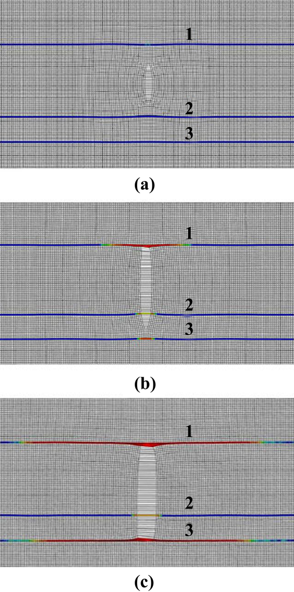
In this section, we simulated a case using the numerical simulation method to investigate the hydraulic fracture propagation behavior when several special layers with different stiffness existed simultaneously. A horizontal well model with a length of about 100 meters was built, as shown in Fig. (11 ). Three special layers numbered 1, 2 and 3 were placed, and they were given different Young’s modulus values, and the assigned values are shown in Table 2. Among the three layers, the Young’s modulus values of layer 1 and layer 3 were higher than that of layer 2. The layer 2 has a same distance to the wellbore with that of layer 1; however, the distance between layer 3 and wellbore is relatively long compared with that of layer 1 or 2. To form a vertical hydraulic fracture perpendicular to the horizontal wellbore, the minimum horizontal stress σh was exerted on the model along the direction which was paralleled to the horizontal wellbore; meanwhile, the maximum horizontal stress σH was forced on the model along the perpendicular direction, and a vertical stress was forced along the vertical direction. The parameters and their assigned values are presented in Table. 2.
 |
Fig. (11) Horizontal well model with a hydraulic fracture approaching the pre-existing different layers. |
4.3.2. Numerical Simulation
The result of the numerical simulation of the fracture propagation when several special layers with different stiffness exist is shown in Fig. (12 ). The result was calculated without remeshing procedure that was an advantage of the simulation method. This figure presents the change of fracture vertical cross-section during propagation at different simulation stages. This view orientation is different from the Figs. (7 and 10). At the first stage (Fig. 12a), the hydraulic fracture began to propagate from the wellbore. At the second simulation stage as shown in Fig. (12b), the fracture crossed the layer 2 and stopped at the layer 1, because the distance between layer 1 and wellbore equals that between layer 2 and wellbore. The crossing phenomenon of fracture is mainly due to the relatively weak stiffness of the layer 2. That is to say, a layer with a weak stiffness may not prevent the fracture propagation. In contrast, the fracture stopped at the layer 1 which has a stronger stiffness. Similar result was obtained at the third simulation stage when the hydraulic fracture reached the layer 3 which also has a relative high stiffness (Fig. 12c). After passing through layer 2, the hydraulic fracture kept growing along the direction toward layer 3 and finally stopped at there. Therefore, the fracture height was limited due to the barrier effect of layers 1 and 3. It can be also found that the hydraulic fracture became wider with the continuance of the simulation. It can be concluded from the above results that the fracture passed through the weak and stopped at the strong. It is due to the reason that the hydraulic fracture propagate when the pressure in the fracture is higher than the rock failure stiffness [20J. Oliver, and A. Huespe, "Continuum approach to material failure in strong discontinuity settings", Comput. Methods Appl. Mech. Eng., vol. 193, pp. 3195-3220, 2004.
[http://dx.doi.org/10.1016/j.cma.2003.07.013] ], and that the pressure is high enough to make the fracture cross the weak layer but not enough to cross the strong layer.
CONCLUSION
Physical simulation experiments on the propagation behavior of hydraulic fracture were carried out with the application of 3D hydraulic fracturing physical simulation system. Meanwhile, numerical simulations were also applied to simulate the propagation behavior of fracture based on the extended finite element method. Several conclusions are summarized as follows.
- With the absence of the interlaminar geostress difference, the lateral and vertical propagation of the fracture occurred, and a fracture with round-shape face was finally presented. Without the interlaminar barrier effect, the growth of the hydraulic fracture is only controlled by the three-dimension principles stress condition.
- With the presence of the interlaminar geostress difference, the fracture height was obviously limited due to the barrier effect of the high stress barrier, and the final shape of the fracture was elliptical.
- When several special layers with different stiffness existed at the same time, the fracture passed through a layer which was relatively weak and stopped at a layer which was relatively strong during the process of fracture propagation.
- The interlaminar geostress difference and layering has considerable effect on propagation behavior of hydraulic fracture, especially the height of the hydraulic fracture.
CONFLICT OF INTEREST
The authors confirm that this article content has no conflict of interest.
ACKNOWLEDGEMENTS
The Key Laboratory of Reservoir Stimulation of China National Petroleum Corporation and Tsinghua University are acknowledged for the support of this work.
REFERENCES
| [1] | C.L. Cipolla, N.R. Warpinski, M.J. Mayerhofer, E.P. Lolon, and M.C. Vincent, The relationship between fracture complexity, reservoir properties, and fracture-treatment design, SPE Annual Technical Conference and Exhibition, 21-24 September 2010, Denver, Colorado. [http://dx.doi.org/10.2118/115769-PA] |
| [2] | W. Kan, and E.O. Jon, "Mechanics analysis of interaction between hydraulic and natural frsctures in shale reservoirs", In: Unconventional Resources Technology Conference, 25-27 August 2014 Denver, Colorado. |
| [3] | H.R. Gu, and E. Siebrits, "Effect of formation modulus contrast on hydraulic fracture height containment", SPE J., vol. 23, pp. 170-176, 2006. |
| [4] | G.M. Gou, and R.Q. Hu, "Controlling gap height and fracture to thin layer", Well Test, vol. 13, pp. 48-53, 2004. |
| [5] | P.Q. Lian, L.S. Cheng, and B. Deng, "Simulation of ground stress field and fracture anticipation with effect of pore pressure", Theor. Appl. Fract. Mech., vol. 56, pp. 34-41, 2011. [http://dx.doi.org/10.1016/j.tafmec.2011.09.004] |
| [6] | J.N. Mohammad, and M. Ali, "Effects of in-situ stress regime and intact rock strength parameters on the hydraulic fracturing", J. Petrol. Sci. Eng., vol. 108, pp. 211-221, 2013. [http://dx.doi.org/10.1016/j.petrol.2013.04.001] |
| [7] | G. Agust, H.S. Trine, L. Belinda, and L.P. Sonja, "Effects of internal structure and local stresses on fracture propagation, deflection, and arrest in fault zones", J. Struct. Geol., vol. 32, pp. 1643-1655, 2010. [http://dx.doi.org/10.1016/j.jsg.2009.08.013] |
| [8] | I.A. Jose, D. Emmanuel, and P.P. Anthony, "Analysis of classical pseudo-3D model for hydraulic fracture with equilibrium height growth across stress barriers", Int. J. Rock Mech. Min. Sci., vol. 47, pp. 625-639, 2010. [http://dx.doi.org/10.1016/j.ijrmms.2010.03.008] |
| [9] | C. Yashwanth, M. Camilo, S. Carl, and R. Chandra, "An experiment investigation into hydraulic fracture propagation under different applied sresses in tight sands using acostic emissions", J. Petrol. Sci. Eng., vol. 108, pp. 151-161, 2013. [http://dx.doi.org/10.1016/j.petrol.2013.01.002] |
| [10] | N.R. Warpinski, J.A. Clark, R.A. Schmidt, and C.W. Huddle, "Laboratory investigation on the effect of In situ stresses on hydraulic fracture containment", SPE J., vol. 22, pp. 333-340, 1982. [http://dx.doi.org/10.2118/9834-PA] |
| [11] | L.W. Teufel, and J.A. Clark, "Hydraulic fracture propagation in layered rock: experimental studies of fracture containment", SPE J., vol. 24, pp. 19-32, 1984. [http://dx.doi.org/10.2118/9878-PA] |
| [12] | T.K. Guo, S.C. Zhang, Z.Q. Qu, T. Zhou, Y.S. Xiao, and J. Gao, "Experimental study of hydraulic fracturing for shale by stimulated reservoir volume", Fuel, vol. 128, pp. 373-380, 2014. [http://dx.doi.org/10.1016/j.fuel.2014.03.029] |
| [13] | Y.P. Li, Y.H. Wang, Y.H. Ding, X. Wang, and L.F. Yang, "Physical and Numerical Simulation of Hydraulic Fracture Initiation and Propagation in Gas Shale", In: SPE Unconventional Resources Conference and Exhibition-Asia Pacific., 11-13 November 2013 Brisbane, Australia,. |
| [14] | T. Mohammadnejad, and A.R. Khoei, "An extended finite element method for hydraulic fracture propagation in deformable porous media with the cohesive crack model", Finite Elem. Anal. Des., vol. 73, pp. 77-95, 2013. [http://dx.doi.org/10.1016/j.finel.2013.05.005] |
| [15] | J. Oliver, A. Huespe, and I. Dias, "Strain localization, strong discontinuities and material fracture: Matches and mismatches", Comput. Methods Appl. Mech. Eng., vol. 241, pp. 323-336, 2012. [http://dx.doi.org/10.1016/j.cma.2012.06.004] |
| [16] | J. Oliver, I. Dias, and A.E. Huespe, "Crack-path field and strain-injection techniques in computational modeling of propagating material failure", Comput. Methods Appl. Mech. Eng., vol. 274, pp. 289-348, 2014. [http://dx.doi.org/10.1016/j.cma.2014.01.008] |
| [17] | T.S. Jaber, "Numerical modeling of hydraulic fracture propagation: Accounting for the effect of stresses on the interaction between hydraulic and parallel natural fractures", Egypt. J. Pet, vol. 22, pp. 557-563, 2013. [http://dx.doi.org/10.1016/j.ejpe.2013.11.010] |
| [18] | G.E. King, "Thirty years of gas shale fracturing: what have we learned?", In: SPE Annual Technical Conference and Exhibition, 19-22 September 2010 Florence, Italy. [http://dx.doi.org/10.2118/133456-MS] |
| [19] | J. Adachi, E. Siebrits, A. Peirce, and J. Desroches, "Computer simulation of hydraulic fractures", Int. J. Rock Mech. Min. Sci., vol. 44, pp. 739-757, 2007. [http://dx.doi.org/10.1016/j.ijrmms.2006.11.006] |
| [20] | J. Oliver, and A. Huespe, "Continuum approach to material failure in strong discontinuity settings", Comput. Methods Appl. Mech. Eng., vol. 193, pp. 3195-3220, 2004. [http://dx.doi.org/10.1016/j.cma.2003.07.013] |